Gene-driven Perturbation (GNP) Knockout Simulation

This tutorial demonstrates how to use the GNP (Gene Network Perturbation) module to perform a silico knockout on mouse Stereo-seq data.

1. Dataset Overview We utilize high-resolution spatial transcriptomics data from the Ma2024 dataset:

Study: Spatial transcriptomic landscape unveils immunoglobulin-associated senescence as a hallmark of aging (Ma, Shuai et al., Cell, 2024).

Biological Context: Analyzing the spatial distribution of senescence markers in the aging mouse brain.

import os
import torch
import numpy as np
import pandas as pd
import scanpy as sc
import gseapy as gp
import anndata as ad
import seaborn as sns
from typing import Optional
from pathlib import Path
import matplotlib.pyplot as plt
from matplotlib.patches import Rectangle
import matplotlib.colors as mcolors
from matplotlib.colors import LinearSegmentedColormap
import sys
sys.path.append("/inspire/ssd/project/sais-lifescience/public/workspace/yangyiwen/Brainbeacon_v2/BrainBeacon/")
from brainbeacon.pipeline.cell_embedding import run_bbcellformer_pipeline
from brainbeacon.pipeline.perturbation import apply_gene_perturbation, inject_cells_into_niche, plot_cosine_to_centroids_with_perturb
from brainbeacon.pipeline.perturbation import analyze_embedding_similarity_change, plot_cosine_to_centroids_with_perturb
from brainbeacon.pipeline.perturbation import analyze_embedding_similarity_change_similarity_niche
from brainbeacon.utils import set_seed
import brainbeacon.configs.config as cfg
from brainbeacon.configs.config_train import config_train as cfg_train
from brainbeacon.utils import compute_density_token, compute_deviation_bin_rapid_v2
from brainbeacon.utils import convert_spatial_to_um, platform_radius_map
import logging
logging.basicConfig(
    level=logging.INFO,  # 或 level=logging.DEBUG
    format='%(asctime)s %(levelname)s %(message)s'
)

import warnings
plt.rcParams["pdf.fonttype"] = 42
warnings.filterwarnings("ignore")
set_seed(42)

Device setup

# Set GPU 
os.environ["CUDA_VISIBLE_DEVICES"] = "0"
device = torch.device("cuda" if torch.cuda.is_available() else "cpu")
print(f"Using device: {device}")
if device.type == "cuda":
    print(f"Using GPU: {torch.cuda.get_device_name(torch.cuda.current_device())}")

# Define base paths and dataset info
out_fig_dir = "/inspire/ssd/project/sais-lifescience/public/yangyiwen_global/Brainbeacon/output/virtual_perturbation/fig4_subfig"
os.makedirs(out_fig_dir, exist_ok=True)

Using device: cuda
Using GPU: NVIDIA H800

Paths and dataset config

Example dataset ()

Path to the processed AnnData object used in this tutorial. The processed file (adata_outer_ensembl.h5ad) can be downloaded directly from: https://drive.google.com/file/d/1-z8J8xiRN0qD0preVQr8cAHKQXuScBp2/view?usp=drive_link Alternatively, the original raw Stereo-seq data can be obtained from the CNGBdb STOmics portal: https://db.cngb.org/stomics/datasets/STDS0000247/data

# =============================================================================
# Dataset and Basic Setup
# =============================================================================
dataset_name = "ma2024aging_cell2niche_niche_inner"
specie = "mouse"  # NOTE: keep original variable name for compatibility
assay = "stereo"

# =============================================================================
# Prior Knowledge / Paths
# =============================================================================
# Base directories
BASE_DIR = Path("/inspire/ssd/project/sais-lifescience/public/yangyiwen_global/Brainbeacon/")

# Sync into cfg (assumes cfg / cfg_train already exist in your notebook/runtime)
cfg.DEFAULT_PATHS["BASE_DIR"] = str(BASE_DIR)
cfg.DEFAULT_PATHS["PRETRAIN_DIR"] = "/inspire/ssd/project/sais-lifescience/public/workspace/yangyiwen/Brainbeacon/bb_PriorKnowledge/"
cfg.DEFAULT_PATHS["PRIOR_DIR"] = cfg.DEFAULT_PATHS["PRETRAIN_DIR"]
cfg.DEFAULT_PATHS["GENE_DICT_PATH"] = (
    "/inspire/ssd/project/sais-lifescience/public/workspace/yangyiwen/Brainbeacon/bb_PriorKnowledge/model_h5ad_1211.h5ad"
)

# Users may start from the raw data and follow their own preprocessing pipeline if desired.
adata_path = BASE_DIR / "data" / "adata_outer_ensembl.h5ad"  # adata_outer_ensembl / adata_inner_ensembl
gene_dict_path = Path(cfg.DEFAULT_PATHS["GENE_DICT_PATH"])
gene_mean_path = Path(
    "/inspire/ssd/project/sais-lifescience/public/yangyiwen_global/Brainbeacon/bb_PriorKnowledge/stereo-seq_gene_nonzero_means_metacell_2.npy"
)

# ESM embedding path
cfg_train["esm_embedding_path"] = (
    "/inspire/ssd/project/sais-lifescience/public/workspace/yangyiwen/Brainbeacon/bb_PriorKnowledge/esm2_embeddings_d5120.pt"
)

# Basic sanity checks (fail fast)
assert adata_path.exists(), f"adata_path not found: {adata_path}"
assert gene_dict_path.exists(), f"gene_dict_path not found: {gene_dict_path}"
assert gene_mean_path.exists(), f"gene_mean_path not found: {gene_mean_path}"
assert Path(cfg_train["esm_embedding_path"]).exists(), f"esm_embedding_path not found: {cfg_train['esm_embedding_path']}"

# =============================================================================
# Pretrained Checkpoints
# =============================================================================
pretrain_dir = BASE_DIR / "pretrained"

bb_ckpt_name = "epoch_0_setp_800000.pt"
cellformer_ckpt_name = "cellformer_epoch99.pt"  # trained on all ma2024aging data
# cellformer_ckpt_name = "cellformer.ckpt"      # CellPLM original checkpoint

bb_ckpt_path = Path("/inspire/ssd/project/sais-lifescience/public/yangyiwen_global/Brainbeacon/bb_PriorKnowledge/epoch_0_step_800000.pt")
cellplm_ckpt_path = Path("/inspire/ssd/project/sais-lifescience/public/yangyiwen_global/Brainbeacon/bb_PriorKnowledge/cellformer_epoch99.pt")

assert bb_ckpt_path.exists(), f"bb_ckpt_path not found: {bb_ckpt_path}"
assert cellplm_ckpt_path.exists(), f"cellplm_ckpt_path not found: {cellplm_ckpt_path}"

# =============================================================================
# Output Naming
# =============================================================================
cd_weight = 0.02
use_hvg = True
n_hvg = 5000

bb_ckpt_tag = bb_ckpt_name.replace(".pt", "").replace(".ckpt", "")
if use_hvg:
    method_name = f"bbcellformer_{bb_ckpt_tag}_hvg{n_hvg}_cd{cd_weight}"
else:
    method_name = f"bbcellformer_{bb_ckpt_tag}_cd{cd_weight}"

output_dir = BASE_DIR / "downstream_tasks" / "virtual_perturbation" / "outputs" / dataset_name / method_name
output_dir.mkdir(parents=True, exist_ok=True)

# =============================================================================
# Load Data and (Optionally) Select Slices
# =============================================================================
full_adata = sc.read_h5ad(str(adata_path))

selected_slices = ["Hippocampus_Y_2_1", "Hippocampus_O_2_1"]

# NOTE: Uncomment if you want to restrict to selected slices
# adata = full_adata[full_adata.obs["slice"].isin(selected_slices)].copy()
adata = full_adata.copy()

# =============================================================================
# Derive Labels
# =============================================================================
def infer_cell_label(slice_name: str) -> Optional[str]:
    """Infer 'Young' / 'Old' from slice naming convention."""
    if slice_name.startswith("Hippocampus_Y"):
        return "Young"
    if slice_name.startswith("Hippocampus_O"):
        return "Old"
    return None  # Unknown slice pattern

# Apply label + batch
adata.obs["cell_label"] = adata.obs["slice"].astype(str).map(infer_cell_label)
adata.obs["batch"] = adata.obs["slice"]

# Enforce categorical type (keeps only 'Young' and 'Old' as known categories)
adata.obs["cell_label"] = pd.Categorical(adata.obs["cell_label"], categories=["Young", "Old"])

DEG_path = "/inspire/ssd/project/sais-lifescience/public/yangyiwen_global/Brainbeacon/bb_PriorKnowledge/1-s2.0-S0092867424012017-mmc2.xlsx" 
#download from supplementary materials of Ma et al., Cell, 2024
DEG_df = pd.read_excel(DEG_path, sheet_name="Hippocampus", skiprows=1)
n_unique_genes = DEG_df["Gene"].str.upper().nunique()
print("Unique gene count:", n_unique_genes)

Unique gene count: 2628

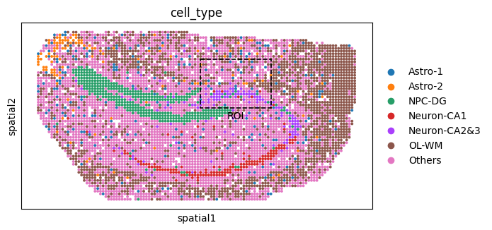
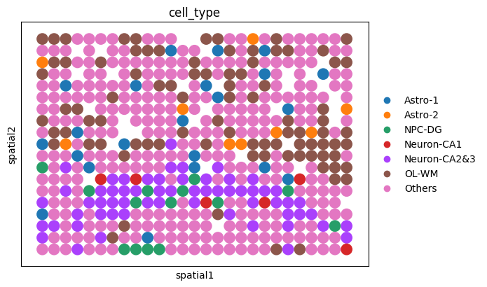
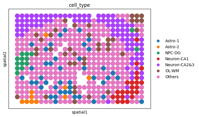
Set ROI

Next, we select regions of interest (ROIs) to further investigate how the perturbation reshapes local cellular niches after gene perturbation. These ROIs enable a focused analysis of spatial and niche-level changes induced by the perturbation.

ol_cells = adata[adata.obs["slice"] == "Hippocampus_O_2_1"].copy()
ol_roi = ol_cells[
    (ol_cells.obsm["spatial"][:, 0] > 60) &    
    (ol_cells.obsm["spatial"][:, 1] > 10) &    
    (ol_cells.obsm["spatial"][:, 0] < 88) &      
    (ol_cells.obsm["spatial"][:, 1] < 30)
].copy()
print(ol_roi)
ol_cells.obs["cell_type"] = ol_cells.obs["cell_type"].astype("category")
categories = ol_cells.obs["cell_type"].cat.categories
ol_roi.obs["cell_type"] = pd.Categorical(
    ol_roi.obs["cell_type"], categories=categories, ordered=True
)

ol_cells.uns["cell_type_colors"] = ol_cells.uns.get(
    "cell_type_colors", sc.pl.palettes.default_20[:len(categories)]
)
ol_roi.uns["cell_type_colors"] = ol_cells.uns["cell_type_colors"]

roi_coords = ol_roi.obsm["spatial"]
xmin, xmax = roi_coords[:, 0].min(), roi_coords[:, 0].max()
ymin, ymax = roi_coords[:, 1].min(), roi_coords[:, 1].max()
xcenter, ycenter = (xmin + xmax) / 2, (ymin + ymax) / 2
os.makedirs(out_fig_dir, exist_ok=True)

fig_ol = sc.pl.spatial(
    ol_cells, color="cell_type", spot_size=1, show=False, return_fig=True
)
ax_ol = fig_ol.axes[0]
rect = Rectangle(
    (xmin, ymin), xmax - xmin, ymax - ymin,
    linewidth=1.2, edgecolor='black', facecolor='none', linestyle='--'
)
ax_ol.add_patch(rect)

ax_ol.text(
    xcenter, ymax + 5, "ROI",
    color='black', fontsize=10, ha='center', va='bottom'
)
fig_roi = sc.pl.spatial(
    ol_roi, color="cell_type", spot_size=1, show=False, return_fig=True
)

AnnData object with n_obs × n_vars = 481 × 20318
    obs: 'x', 'y', 'cell_type', 'n_genes_by_counts', 'log1p_n_genes_by_counts', 'total_counts', 'log1p_total_counts', 'pct_counts_in_top_50_genes', 'pct_counts_in_top_100_genes', 'pct_counts_in_top_200_genes', 'pct_counts_in_top_500_genes', 'total_counts_mito', 'log1p_total_counts_mito', 'pct_counts_mito', 'clusters', 'cell_label', 'slice', 'species', 'age_group', 'batch'
    var: 'gene_symbol', 'ensembl', 'human_symbol', 'human_ensembl'
    obsm: 'X_pca', 'X_umap', 'spatial'
    layers: 'lognorm', 'raw_count'

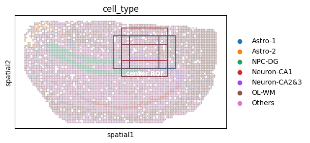
# This snippet visualizes ROI “jittering” (window shifting) by drawing multiple shifted ROI boxes
# on the same spatial plot, illustrating how small window movements can improve robustness.

fig_ol = sc.pl.spatial(
    ol_cells,
    color="cell_type",
    spot_size=1,
    show=False,
    return_fig=True,
)
ax_ol = fig_ol.axes[0]

# Make all cell-type colors more muted (blend with gray) for better ROI contrast
gray = np.array([0.5, 0.5, 0.5, 1.0])
for c in ax_ol.collections:
    facecolors = c.get_facecolor()
    c.set_facecolor(0.5 * facecolors + 0.5 * gray)
    c.set_alpha(0.5)

# Base ROI coordinates and a set of small shifts (jitter)
ol_base_x, ol_base_y = (60, 88), (10, 30)
shifts = [
    (0, 0),
    (5, 0),
    (-5, 0),
    (0, 5),
    (0, -5),
]

# Color gradient for shifted ROI boxes
start_color = "#145583"
end_color = "#A13939"
cmap = LinearSegmentedColormap.from_list("blue_red", [start_color, end_color])
colors = [cmap(i / (len(shifts) - 1)) for i in range(len(shifts))]

# Draw ROI boxes with different shifts
for i, (dx, dy) in enumerate(shifts):
    xmin, xmax = ol_base_x[0] + dx, ol_base_x[1] + dx
    ymin, ymax = ol_base_y[0] + dy, ol_base_y[1] + dy

    ax_ol.add_patch(
        Rectangle(
            (xmin, ymin),
            xmax - xmin,
            ymax - ymin,
            linewidth=1.4,
            edgecolor=colors[i],
            facecolor="none",
            linestyle="-",
            alpha=0.95,
        )
    )

# Annotate the center ROI
ax_ol.text(
    np.mean(ol_base_x),
    ol_base_y[1] + 5,
    "center ROI",
    color="white",
    fontsize=9,
    weight="bold",
    ha="center",
    va="bottom",
)

plt.tight_layout()
# plt.savefig(f"{out_fig_dir}/c2n_ol_cells_with_multiple_roi_boxes.pdf", bbox_inches="tight")
plt.show()

# === Matplotlib settings (ensure editable text in PDF/SVG) ===
warnings.filterwarnings("ignore")
logging.getLogger('matplotlib.font_manager').disabled = True

plt.rcParams['pdf.fonttype'] = 42
plt.rcParams['ps.fonttype']  = 42
plt.rcParams['svg.fonttype'] = 'none'
plt.rcParams['font.sans-serif'] = ['Arial']
plt.rcParams['font.family'] = 'sans-serif'

# === Ensure output directory ===
os.makedirs(out_fig_dir, exist_ok=True)

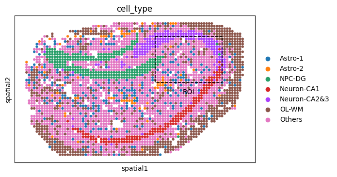
# === Step 1: subset slice ===
adata_Y = adata[adata.obs["slice"] == "Hippocampus_Y_2_1"].copy()

# === Step 2: coordinates ===
x = adata_Y.obsm["spatial"][:, 0]
y = adata_Y.obsm["spatial"][:, 1]
print(f"x: {x.min():.1f} ~ {x.max():.1f}, y: {y.min():.1f} ~ {y.max():.1f}")

# === Step 3: ROI bounds (x in (60, 88), y in (10, 30)) ===
roi_mask = (x > 50) & (x < 78) & (y > 5) & (y < 25)
y_roi = adata_Y[roi_mask].copy()
print(f"ROI cells: {y_roi.n_obs}")

# === Step 4: sync categories & colors ===
adata_Y.obs["cell_type"] = adata_Y.obs["cell_type"].astype("category")
cats = adata_Y.obs["cell_type"].cat.categories
y_roi.obs["cell_type"] = pd.Categorical(y_roi.obs["cell_type"], categories=cats, ordered=True)

adata_Y.uns["cell_type_colors"] = adata_Y.uns.get(
    "cell_type_colors", sc.pl.palettes.default_20[:len(cats)]
)
y_roi.uns["cell_type_colors"] = adata_Y.uns["cell_type_colors"]

# === Step 5a: full view with ROI box ===
fig1 = sc.pl.spatial(adata_Y, color="cell_type", spot_size=1, show=False, return_fig=True)

# Add dashed ROI box
roi_xy = y_roi.obsm["spatial"]
xmin, xmax = roi_xy[:, 0].min(), roi_xy[:, 0].max()
ymin, ymax = roi_xy[:, 1].min(), roi_xy[:, 1].max()
xcenter, ycenter = (xmin + xmax) / 2, (ymin + ymax) / 2

ax = fig1.axes[0]
rect = Rectangle((xmin, ymin), xmax - xmin, ymax - ymin,
                 linewidth=1.2, edgecolor='black', facecolor='none', linestyle='--')
ax.add_patch(rect)
ax.text(xcenter, ymax + 5, "ROI", color='black', fontsize=10, ha='center', va='bottom')
# === Step 5b: ROI-only ===
fig2 = sc.pl.spatial(y_roi, color="cell_type", spot_size=1, show=False, return_fig=True)

x: 1.0 ~ 85.0, y: 1.0 ~ 52.0
ROI cells: 495

ol_roi.obs["brain_region"] = ol_roi.obs["slice"]
ol_roi.obs["brain_region_main"] = ol_roi.obs["slice"]
ol_roi.obsm["spatial"] = ol_roi.obsm["spatial"].astype(np.float32)
ol_roi = compute_deviation_bin_rapid_v2(ol_roi)
ol_roi = convert_spatial_to_um(ol_roi, "STEREO")
radius = platform_radius_map.get("STEREO_bin", 8)
ol_roi, _ = compute_density_token(ol_roi, radius)

y_roi.obs["brain_region"] = y_roi.obs["slice"]
y_roi.obs["brain_region_main"] = y_roi.obs["slice"]
y_roi.obsm["spatial"] = y_roi.obsm["spatial"].astype(np.float32)
y_roi = compute_deviation_bin_rapid_v2(y_roi)
y_roi = convert_spatial_to_um(y_roi, "STEREO")
radius = platform_radius_map.get("STEREO_bin", 8)
y_roi, _ = compute_density_token(y_roi, radius)

adata_fov_OL = ad.concat([ol_roi, y_roi], join="outer")
adata_fov_OL.var = adata.var.loc[adata_fov_OL.var_names].copy()
output_prefix_ori = "original"
adata_fov_OL.obs["split"] = "train"
os.makedirs(output_dir, exist_ok=True)
ori_input_adata_path = os.path.join(output_dir, f"{output_prefix_ori}_input.h5ad")
adata_fov_OL.write(ori_input_adata_path)
print(f"Saved selected slices to: {ori_input_adata_path}")

Saved selected slices to: /inspire/ssd/project/sais-lifescience/public/yangyiwen_global/Brainbeacon/downstream_tasks/virtual_perturbation/outputs/ma2024aging_cell2niche_niche_inner/bbcellformer_epoch_0_setp_800000_hvg5000_cd0.02/original_input.h5ad

print(ol_roi)
print(y_roi)
print(adata)
print(adata_fov_OL)

AnnData object with n_obs × n_vars = 481 × 20318
    obs: 'x', 'y', 'cell_type', 'n_genes_by_counts', 'log1p_n_genes_by_counts', 'total_counts', 'log1p_total_counts', 'pct_counts_in_top_50_genes', 'pct_counts_in_top_100_genes', 'pct_counts_in_top_200_genes', 'pct_counts_in_top_500_genes', 'total_counts_mito', 'log1p_total_counts_mito', 'pct_counts_mito', 'clusters', 'cell_label', 'slice', 'species', 'age_group', 'batch', 'brain_region', 'brain_region_main', 'slice_brain_area', 'density_token'
    var: 'gene_symbol', 'ensembl', 'human_symbol', 'human_ensembl'
    uns: 'cell_type_colors'
    obsm: 'X_pca', 'X_umap', 'spatial', 'deviation_bin', 'neighbor_gene_distribution', 'spatial_um'
    layers: 'lognorm', 'raw_count'
AnnData object with n_obs × n_vars = 495 × 20318
    obs: 'x', 'y', 'cell_type', 'n_genes_by_counts', 'log1p_n_genes_by_counts', 'total_counts', 'log1p_total_counts', 'pct_counts_in_top_50_genes', 'pct_counts_in_top_100_genes', 'pct_counts_in_top_200_genes', 'pct_counts_in_top_500_genes', 'total_counts_mito', 'log1p_total_counts_mito', 'pct_counts_mito', 'clusters', 'cell_label', 'slice', 'species', 'age_group', 'batch', 'brain_region', 'brain_region_main', 'slice_brain_area', 'density_token'
    var: 'gene_symbol', 'ensembl', 'human_symbol', 'human_ensembl'
    uns: 'cell_type_colors'
    obsm: 'X_pca', 'X_umap', 'spatial', 'deviation_bin', 'neighbor_gene_distribution', 'spatial_um'
    layers: 'lognorm', 'raw_count'
AnnData object with n_obs × n_vars = 57140 × 20318
    obs: 'x', 'y', 'cell_type', 'n_genes_by_counts', 'log1p_n_genes_by_counts', 'total_counts', 'log1p_total_counts', 'pct_counts_in_top_50_genes', 'pct_counts_in_top_100_genes', 'pct_counts_in_top_200_genes', 'pct_counts_in_top_500_genes', 'total_counts_mito', 'log1p_total_counts_mito', 'pct_counts_mito', 'clusters', 'cell_label', 'slice', 'species', 'age_group', 'batch'
    var: 'gene_symbol', 'ensembl', 'human_symbol', 'human_ensembl'
    obsm: 'X_pca', 'X_umap', 'spatial'
    layers: 'lognorm', 'raw_count'
AnnData object with n_obs × n_vars = 976 × 20318
    obs: 'x', 'y', 'cell_type', 'n_genes_by_counts', 'log1p_n_genes_by_counts', 'total_counts', 'log1p_total_counts', 'pct_counts_in_top_50_genes', 'pct_counts_in_top_100_genes', 'pct_counts_in_top_200_genes', 'pct_counts_in_top_500_genes', 'total_counts_mito', 'log1p_total_counts_mito', 'pct_counts_mito', 'clusters', 'cell_label', 'slice', 'species', 'age_group', 'batch', 'brain_region', 'brain_region_main', 'slice_brain_area', 'density_token', 'split'
    var: 'gene_symbol', 'ensembl', 'human_symbol', 'human_ensembl'
    obsm: 'X_pca', 'X_umap', 'spatial', 'deviation_bin', 'neighbor_gene_distribution', 'spatial_um'
    layers: 'lognorm', 'raw_count'

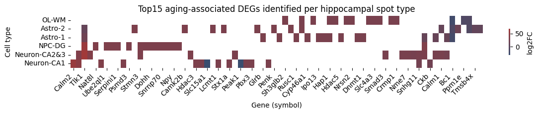
# This snippet visualizes the overlap between a curated DEG list (DEG_df)
# and the aging-associated gene set provided by Ma et al., Cell (2024),
# by computing cell type–specific Old vs Young DEGs and summarizing the top genes as a log2FC heatmap.

unique_genes_global = set(DEG_df["Gene"].unique())
print("Unique gene count (global):", len(unique_genes_global))

adata_no_others = adata_fov_OL[adata_fov_OL.obs["cell_type"] != "Others", :].copy()

adata_no_others.obs["group"] = adata_no_others.obs["slice"].map(
    {
        "Hippocampus_O_2_1": "Old",
        "Hippocampus_Y_2_1": "Young",
    }
)

pval_thr = 0.01

deg_results = {}
all_top_genes = {}

for ct in adata_no_others.obs["cell_type"].unique():
    print(f"Processing {ct}...")

    adata_ct = adata_no_others[adata_no_others.obs["cell_type"] == ct, :].copy()
    if adata_ct.n_obs < 5:
        print(f"  Skip {ct} (too few cells)")
        continue

    sc.tl.rank_genes_groups(
        adata_ct,
        groupby="group",
        reference="Young",
        method="wilcoxon",
    )
    deg_df = sc.get.rank_genes_groups_df(adata_ct, group="Old")

    id_to_symbol = adata_ct.var["gene_symbol"].to_dict()
    deg_df["gene_symbol"] = deg_df["names"].map(id_to_symbol)

    deg_df = deg_df[deg_df["pvals"] < pval_thr].copy()
    if deg_df.empty:
        continue

    deg_df = deg_df[deg_df["gene_symbol"].isin(unique_genes_global)]
    if deg_df.empty:
        continue

    deg_df = deg_df.sort_values(by="logfoldchanges", key=abs, ascending=False)

    # Top 15 genes per cell type
    top_genes = deg_df.head(15)
    top_symbols = top_genes["gene_symbol"].tolist()

    all_top_genes[ct] = top_symbols
    deg_results[ct] = top_genes.set_index("gene_symbol")["logfoldchanges"]

logfc_mat = pd.DataFrame(deg_results).T

gene_abs_mean = logfc_mat.abs().mean(axis=0)
final_gene_order = gene_abs_mean.sort_values(ascending=False).index.tolist()
logfc_mat = logfc_mat[final_gene_order]

cmap = LinearSegmentedColormap.from_list("custom", ["#145583", "#A13939"])

n_celltypes = logfc_mat.shape[0]
fig_height = max(2, 0.4 * n_celltypes)

plt.figure(figsize=(12, fig_height))
sns.heatmap(
    logfc_mat,
    cmap=cmap,
    center=0,
    annot=False,
    cbar_kws={
        "shrink": 0.5,
        "label": "log2FC",
    },
)
plt.title("Top15 aging-associated DEGs identified per hippocampal spot type")
plt.ylabel("Cell type")
plt.xlabel("Gene (symbol)")
plt.xticks(rotation=45, ha="right")
plt.tight_layout()
# plt.savefig(f"{out_fig_dir}/Top15 aging-associated DEGs_heatmap.pdf", bbox_inches="tight")
plt.show()

Unique gene count (global): 2628
Processing OL-WM...
WARNING: It seems you use rank_genes_groups on the raw count data. Please logarithmize your data before calling rank_genes_groups.
Processing Astro-2...
WARNING: It seems you use rank_genes_groups on the raw count data. Please logarithmize your data before calling rank_genes_groups.
Processing Astro-1...
WARNING: It seems you use rank_genes_groups on the raw count data. Please logarithmize your data before calling rank_genes_groups.
Processing NPC-DG...
WARNING: It seems you use rank_genes_groups on the raw count data. Please logarithmize your data before calling rank_genes_groups.
Processing Neuron-CA2&3...
WARNING: It seems you use rank_genes_groups on the raw count data. Please logarithmize your data before calling rank_genes_groups.
Processing Neuron-CA1...
WARNING: It seems you use rank_genes_groups on the raw count data. Please logarithmize your data before calling rank_genes_groups.

Run Original Inference

This step constructs the baseline (unperturbed) reference by running inference kon the original data, which serves as the control condition for all subsequent perturbation analyses.

adata_ori = run_bbcellformer_pipeline(
    adata_path=ori_input_adata_path,
    specie=specie,
    assay=assay,
    gene_dict_path=gene_dict_path,
    gene_mean_path=gene_mean_path,
    bb_ckpt_path=bb_ckpt_path,
    cellplm_ckpt_path=cellplm_ckpt_path,
    output_dir=output_dir,
    output_prefix=output_prefix_ori,
    config_train=cfg_train,
    n_hvg=n_hvg,
    cd_weight=cd_weight,
    use_hvg=use_hvg,
    weight_mode="expression",
    use_batch=False,
    use_spatial=True,
    force_tokenize=True,
    do_fit=True,  # recommended to set to True for original reconstruction
    device=device,
    fit_epochs=100,
)
print("Original reconstruction complete. Embeddings and model saved.")
print("adata_ori:", adata_ori)

ori_result_adata_path = os.path.join(output_dir, f"{output_prefix_ori}_result.h5ad")
adata_ori.write(ori_result_adata_path)
print(f"Original result adata saved to: {ori_result_adata_path}")

Forcing re-tokenization: clearing existing .parquet files and token folders...
No existing tokenized files found. Running tokenization...
path to process: /inspire/ssd/project/sais-lifescience/public/yangyiwen_global/Brainbeacon/downstream_tasks/virtual_perturbation/outputs/ma2024aging_cell2niche_niche_inner/bbcellformer_epoch_0_setp_800000_hvg5000_cd0.02/original_input.h5ad
before quality control adata shape: (976, 20318)
After HVG (5000) selection: (976, 5000)
Computing cell density...
compute_density_token time:  0.0038423975308736163 min
Begin processing: /inspire/ssd/project/sais-lifescience/public/yangyiwen_global/Brainbeacon/downstream_tasks/virtual_perturbation/outputs/ma2024aging_cell2niche_niche_inner/bbcellformer_epoch_0_setp_800000_hvg5000_cd0.02/original_bb_token_dir/tokens-0000.parquet
Table shape from parquet = 976
Preprocessing time: 0.12 minutes
Loaded pretrain_model checkpoint: /inspire/ssd/project/sais-lifescience/public/yangyiwen_global/Brainbeacon/bb_PriorKnowledge/epoch_0_step_800000.pt
obs_names and pred_indices are in the same order.
Embeddings saved to /inspire/ssd/project/sais-lifescience/public/yangyiwen_global/Brainbeacon/downstream_tasks/virtual_perturbation/outputs/ma2024aging_cell2niche_niche_inner/bbcellformer_epoch_0_setp_800000_hvg5000_cd0.02/original_bb_embeddings.npz
Time cost:  0.561520532766978
BB inference complete. Saved to: /inspire/ssd/project/sais-lifescience/public/yangyiwen_global/Brainbeacon/downstream_tasks/virtual_perturbation/outputs/ma2024aging_cell2niche_niche_inner/bbcellformer_epoch_0_setp_800000_hvg5000_cd0.02/original_bb_embeddings.npz
[INFO] Using explicitly provided CellFormer checkpoint: /inspire/ssd/project/sais-lifescience/public/yangyiwen_global/Brainbeacon/bb_PriorKnowledge/cellformer_epoch99.pt
********** gene list size: 92076 **********
********** loading skip parameters: set() **********
After filtering, 20316 genes remain.
Epoch 0 | Train loss: 19754.3462 | Valid loss: 20418.4263
Epoch 1 | Train loss: 17814.4434 | Valid loss: 17169.4941
Epoch 2 | Train loss: 15183.4585 | Valid loss: 13781.2520
Epoch 3 | Train loss: 11961.5400 | Valid loss: 10546.7905
Epoch 4 | Train loss: 9717.5762 | Valid loss: 8113.6162
Epoch 5 | Train loss: 7772.9041 | Valid loss: 7407.3206
Epoch 6 | Train loss: 7313.2432 | Valid loss: 7223.4465
Epoch 7 | Train loss: 7241.3916 | Valid loss: 7218.8459
Epoch 8 | Train loss: 7173.7888 | Valid loss: 7216.5046
Epoch 9 | Train loss: 7202.7556 | Valid loss: 7213.8367
Epoch 10 | Train loss: 7336.0952 | Valid loss: 7210.1489
Epoch 11 | Train loss: 7185.5908 | Valid loss: 7206.6870
Epoch 12 | Train loss: 7419.1924 | Valid loss: 7202.9348
Epoch 13 | Train loss: 7183.8896 | Valid loss: 7198.8628
Epoch 14 | Train loss: 7136.3804 | Valid loss: 7195.8555
Epoch 15 | Train loss: 7220.1282 | Valid loss: 7191.6562
Epoch 16 | Train loss: 7207.6970 | Valid loss: 7188.3438
Epoch 17 | Train loss: 7234.3596 | Valid loss: 7184.7644
Epoch 18 | Train loss: 7086.0078 | Valid loss: 7180.6450
Epoch 19 | Train loss: 7186.0859 | Valid loss: 7176.7720
Epoch 20 | Train loss: 7314.2183 | Valid loss: 7171.2444
Epoch 21 | Train loss: 7039.5352 | Valid loss: 7162.0793
Epoch 22 | Train loss: 7108.5981 | Valid loss: 7162.9985
Epoch 23 | Train loss: 7162.5605 | Valid loss: 7153.5894
Epoch 24 | Train loss: 7172.5879 | Valid loss: 7153.8652
Epoch 25 | Train loss: 7164.2371 | Valid loss: 7147.8079
Epoch 26 | Train loss: 7072.0237 | Valid loss: 7142.3708
Epoch 27 | Train loss: 7235.6038 | Valid loss: 7143.4756
Epoch 28 | Train loss: 7169.2344 | Valid loss: 7139.4495
Epoch 29 | Train loss: 7099.4167 | Valid loss: 7131.1633
Epoch 30 | Train loss: 7199.0378 | Valid loss: 7129.1655
Epoch 31 | Train loss: 7277.7117 | Valid loss: 7124.9893
Epoch 32 | Train loss: 7105.2947 | Valid loss: 7119.7693
Epoch 33 | Train loss: 7005.3721 | Valid loss: 7117.6055
Epoch 34 | Train loss: 7091.3821 | Valid loss: 7112.8389
Epoch 35 | Train loss: 7042.4587 | Valid loss: 7108.1072
Epoch 36 | Train loss: 7141.8374 | Valid loss: 7103.7412
Epoch 37 | Train loss: 7117.8672 | Valid loss: 7099.7349
Epoch 38 | Train loss: 7023.4429 | Valid loss: 7094.4160
Epoch 39 | Train loss: 7052.7529 | Valid loss: 7089.2034
Epoch 40 | Train loss: 7008.0156 | Valid loss: 7084.6860
Epoch 41 | Train loss: 7140.2300 | Valid loss: 7080.0132
Epoch 42 | Train loss: 7011.5356 | Valid loss: 7075.1487
Epoch 43 | Train loss: 7187.6658 | Valid loss: 7070.1191
Epoch 44 | Train loss: 7162.8506 | Valid loss: 7064.9451
Epoch 45 | Train loss: 6939.2012 | Valid loss: 7059.8992
Epoch 46 | Train loss: 6983.5208 | Valid loss: 7054.8860
Epoch 47 | Train loss: 7025.1587 | Valid loss: 7049.5667
Epoch 48 | Train loss: 7034.9082 | Valid loss: 7044.4058
Epoch 49 | Train loss: 7024.4331 | Valid loss: 7039.7097
Epoch 50 | Train loss: 6972.8816 | Valid loss: 7034.4268
Epoch 51 | Train loss: 7055.8447 | Valid loss: 7029.2246
Epoch 52 | Train loss: 7000.6719 | Valid loss: 7024.8030
Epoch 53 | Train loss: 7098.1392 | Valid loss: 7020.6677
Epoch 54 | Train loss: 6944.7014 | Valid loss: 7016.8149
Epoch 55 | Train loss: 6951.4971 | Valid loss: 7012.1958
Epoch 56 | Train loss: 7022.1548 | Valid loss: 7006.7651
Epoch 57 | Train loss: 7018.0371 | Valid loss: 7002.4963
Epoch 58 | Train loss: 7031.2852 | Valid loss: 6998.7092
Epoch 59 | Train loss: 6929.1497 | Valid loss: 6995.4094
Epoch 60 | Train loss: 7036.0046 | Valid loss: 6991.7349
Epoch 61 | Train loss: 6976.5562 | Valid loss: 6987.4307
Epoch 62 | Train loss: 6927.7271 | Valid loss: 6983.2922
Epoch 63 | Train loss: 7000.6475 | Valid loss: 6979.1929
Epoch 64 | Train loss: 7093.4644 | Valid loss: 6975.1660
Epoch 65 | Train loss: 6926.8337 | Valid loss: 6971.0662
Epoch 66 | Train loss: 6851.7664 | Valid loss: 6966.5933
Epoch 67 | Train loss: 7034.8625 | Valid loss: 6962.4028
Epoch 68 | Train loss: 6878.9407 | Valid loss: 6958.4116
Epoch 69 | Train loss: 6999.4861 | Valid loss: 6954.3601
Epoch 70 | Train loss: 7005.4026 | Valid loss: 6950.0229
Epoch 71 | Train loss: 6938.2839 | Valid loss: 6945.4683
Epoch 72 | Train loss: 6919.0798 | Valid loss: 6941.2195
Epoch 73 | Train loss: 6975.8445 | Valid loss: 6937.4939
Epoch 74 | Train loss: 6994.0798 | Valid loss: 6933.9502
Epoch 75 | Train loss: 7068.9517 | Valid loss: 6930.2771
Epoch 76 | Train loss: 6771.8110 | Valid loss: 6926.0325
Epoch 77 | Train loss: 7116.1509 | Valid loss: 6922.0166
Epoch 78 | Train loss: 6822.9250 | Valid loss: 6918.2007
Epoch 79 | Train loss: 6880.4580 | Valid loss: 6914.6807
Epoch 80 | Train loss: 6768.1404 | Valid loss: 6911.0068
Epoch 81 | Train loss: 6660.9297 | Valid loss: 6906.6199
Epoch 82 | Train loss: 6833.1191 | Valid loss: 6902.5620
Epoch 83 | Train loss: 6880.1580 | Valid loss: 6898.6567
Epoch 84 | Train loss: 6931.6531 | Valid loss: 6895.2039
Epoch 85 | Train loss: 6855.9238 | Valid loss: 6891.3103
Epoch 86 | Train loss: 6990.7883 | Valid loss: 6887.4758
Epoch 87 | Train loss: 6835.4873 | Valid loss: 6883.1985
Epoch 88 | Train loss: 6870.0300 | Valid loss: 6879.4187
Epoch 89 | Train loss: 6879.7190 | Valid loss: 6875.8972
Epoch 90 | Train loss: 6798.6077 | Valid loss: 6872.0786
Epoch 91 | Train loss: 6907.3708 | Valid loss: 6868.3650
Epoch 92 | Train loss: 6903.1123 | Valid loss: 6864.8435
Epoch 93 | Train loss: 6883.6060 | Valid loss: 6861.2314
Epoch 94 | Train loss: 6739.6294 | Valid loss: 6857.4692
Epoch 95 | Train loss: 6816.6841 | Valid loss: 6853.9160
Epoch 96 | Train loss: 6855.8743 | Valid loss: 6850.5432
Epoch 97 | Train loss: 6965.2151 | Valid loss: 6847.2788
Epoch 98 | Train loss: 6803.6355 | Valid loss: 6843.8608
Epoch 99 | Train loss: 6832.2544 | Valid loss: 6840.0640
After filtering, 20316 genes remain.
Model saved to /inspire/ssd/project/sais-lifescience/public/yangyiwen_global/Brainbeacon/downstream_tasks/virtual_perturbation/outputs/ma2024aging_cell2niche_niche_inner/bbcellformer_epoch_0_setp_800000_hvg5000_cd0.02/original_cellformer.pt
Embeddings saved to /inspire/ssd/project/sais-lifescience/public/yangyiwen_global/Brainbeacon/downstream_tasks/virtual_perturbation/outputs/ma2024aging_cell2niche_niche_inner/bbcellformer_epoch_0_setp_800000_hvg5000_cd0.02/original_embeddings.npz
Original reconstruction complete. Embeddings and model saved.
adata_ori: AnnData object with n_obs × n_vars = 976 × 20316
    obs: 'x', 'y', 'cell_type', 'n_genes_by_counts', 'log1p_n_genes_by_counts', 'total_counts', 'log1p_total_counts', 'pct_counts_in_top_50_genes', 'pct_counts_in_top_100_genes', 'pct_counts_in_top_200_genes', 'pct_counts_in_top_500_genes', 'total_counts_mito', 'log1p_total_counts_mito', 'pct_counts_mito', 'clusters', 'cell_label', 'slice', 'species', 'age_group', 'batch', 'brain_region', 'brain_region_main', 'slice_brain_area', 'density_token', 'split', 'platform', 'valid_split', 'x_FOV_px', 'y_FOV_px'
    var: 'gene_symbol', 'ensembl', 'human_symbol', 'human_ensembl'
    obsm: 'X_pca', 'X_umap', 'deviation_bin', 'neighbor_gene_distribution', 'spatial', 'spatial_um', 'bb_emb', 'X_emb', 'X_pred'
    layers: 'lognorm', 'raw_count'
Original result adata saved to: /inspire/ssd/project/sais-lifescience/public/yangyiwen_global/Brainbeacon/downstream_tasks/virtual_perturbation/outputs/ma2024aging_cell2niche_niche_inner/bbcellformer_epoch_0_setp_800000_hvg5000_cd0.02/original_result.h5ad

Example perturbation (in silico knockout) and pre/post effect evaluation

This module demonstrates an in silico gene knockout workflow on a specific cell population. Here we use OL-WM cells as an example and knock out Meg3 in the Old mouse hippocampus slice (“Hippocampus_O_2_1”) by setting its expression to 0 in the selected cells.

After perturbation, we evaluate how the niche-level representation/distribution changes by comparing pre- vs post-perturbation metrics, including:

• Cosine similarity

• Euclidean distance

• Wasserstein distance (EMD)

• Maximum Mean Discrepancy (MMD)

You can adapt this example by changing:

• gene_list: the gene(s) you want to perturb (e.g., [“Igkc”], [“Apoe”], …)

• filter_by: the target slice and/or cell type (e.g., other slices, other cell types)

• mode: perturbation type such as “knockout” or other supported modes in your function

• multiplier: optional scaling factor if you use a non-knockout perturbation mode

perturbed_adata_final, perturbed_cells_final = apply_gene_perturbation(
    adata=adata_fov_OL,
    gene_list=["Meg3"],  # Replace with genes of interest, e.g., ["Igkc"] or multiple genes ["GeneA", "GeneB"]
    mode="knockout",  # Perturbation mode; replace with other supported modes if needed
    filter_by={
        "slice": "Hippocampus_O_2_1",  # Replace with a different slice if you want to target another region/sample
        "cell_type": "OL-WM",          # Replace with a different cell type (or other metadata keys) as your target
    },
    multiplier=None,  # Optional; set if using a scaling-based perturbation mode (e.g., suppression/overexpression)
)
print(f"Perturbed {len(perturbed_cells_final)} cells: set expression of target gene(s) to 0.")

# Save perturbed input data
output_prefix_perturb = "ko_old_final"
perturb_input_adata_path = os.path.join(output_dir, f"{output_prefix_perturb}_input.h5ad")
perturbed_adata_final.write(perturb_input_adata_path)
print(f"Perturbed {len(perturbed_cells_final)} cells: set expression of target gene(s) to 0.")

# Save perturbed input data
output_prefix_perturb = "ko_old_final"
perturb_input_adata_path = os.path.join(output_dir, f"{output_prefix_perturb}_input.h5ad")
perturbed_adata_final.write(perturb_input_adata_path)
print(f"Perturbed input adata saved to: {perturb_input_adata_path}")

# ========== Run Perturbation Inference ==========
cellplm_ckpt_path = os.path.join(output_dir, f"{output_prefix_ori}_cellformer.pt")
adata_perturb_final = run_bbcellformer_pipeline(
    adata_path=perturb_input_adata_path,
    specie=specie,
    assay=assay,
    gene_dict_path=gene_dict_path,
    gene_mean_path=gene_mean_path,
    bb_ckpt_path=bb_ckpt_path,
    cellplm_ckpt_path=cellplm_ckpt_path,
    output_dir=output_dir,
    output_prefix=output_prefix_perturb,
    config_train=cfg_train,
    n_hvg=n_hvg,
    cd_weight=cd_weight,
    use_hvg=use_hvg,
    use_batch=False,
    use_spatial=True,
    weight_mode="expression",
    force_tokenize=True,
    do_fit=False,
    fit_epochs=10,
    device=device
)
print("Perturbation reconstruction complete. Embeddings and model saved.")
print("adata_perturb:", adata_perturb_final)

perturb_result_adata_path = os.path.join(output_dir, f"{output_prefix_perturb}_result.h5ad")
adata_perturb_final.write(perturb_result_adata_path)
print(f"Perturbation result adata saved to: {perturb_result_adata_path}")

# ========== Analyze Embedding Similarity Change ==========
target_slice_young = "Hippocampus_Y_2_1"
target_slice_old = "Hippocampus_O_2_1"
target_celltype = "OL-WM"

print("\n>>> Analyzing embedding similarity between old and young cells...")
sim_ko_meg3 = analyze_embedding_similarity_change(
    adata_ori_result=adata_ori,
    adata_perturb_result=adata_perturb_final,
    target_slice_young=target_slice_young,
    target_slice_old=target_slice_old,
    target_celltype=target_celltype,
    embedding_key="X_emb"
)
sim_ko_meg3_niche = analyze_embedding_similarity_change_similarity_niche(
    adata_ori_result=adata_ori,
    adata_perturb_result=adata_perturb_final,
    target_slice_young=target_slice_young,
    target_slice_old=target_slice_old,
    target_celltype=target_celltype,
    embedding_key="X_emb"
)

Perturbed 88 cells: set expression of target gene(s) to 0.
Perturbed 88 cells: set expression of target gene(s) to 0.
Perturbed input adata saved to: /inspire/ssd/project/sais-lifescience/public/yangyiwen_global/Brainbeacon/downstream_tasks/virtual_perturbation/outputs/ma2024aging_cell2niche_niche_inner/bbcellformer_epoch_0_setp_800000_hvg5000_cd0.02/ko_old_final_input.h5ad
Forcing re-tokenization: clearing existing .parquet files and token folders...
No existing tokenized files found. Running tokenization...
path to process: /inspire/ssd/project/sais-lifescience/public/yangyiwen_global/Brainbeacon/downstream_tasks/virtual_perturbation/outputs/ma2024aging_cell2niche_niche_inner/bbcellformer_epoch_0_setp_800000_hvg5000_cd0.02/ko_old_final_input.h5ad
before quality control adata shape: (976, 20318)
After HVG (5000) selection: (976, 5000)
Computing cell density...
compute_density_token time:  0.003927679856618246 min
Begin processing: /inspire/ssd/project/sais-lifescience/public/yangyiwen_global/Brainbeacon/downstream_tasks/virtual_perturbation/outputs/ma2024aging_cell2niche_niche_inner/bbcellformer_epoch_0_setp_800000_hvg5000_cd0.02/ko_old_final_bb_token_dir/tokens-0000.parquet
Table shape from parquet = 976
Preprocessing time: 0.05 minutes
Loaded pretrain_model checkpoint: /inspire/ssd/project/sais-lifescience/public/yangyiwen_global/Brainbeacon/bb_PriorKnowledge/epoch_0_step_800000.pt
obs_names and pred_indices are in the same order.
Embeddings saved to /inspire/ssd/project/sais-lifescience/public/yangyiwen_global/Brainbeacon/downstream_tasks/virtual_perturbation/outputs/ma2024aging_cell2niche_niche_inner/bbcellformer_epoch_0_setp_800000_hvg5000_cd0.02/ko_old_final_bb_embeddings.npz
Time cost:  0.2840085466702779
BB inference complete. Saved to: /inspire/ssd/project/sais-lifescience/public/yangyiwen_global/Brainbeacon/downstream_tasks/virtual_perturbation/outputs/ma2024aging_cell2niche_niche_inner/bbcellformer_epoch_0_setp_800000_hvg5000_cd0.02/ko_old_final_bb_embeddings.npz
[INFO] Using explicitly provided CellFormer checkpoint: /inspire/ssd/project/sais-lifescience/public/yangyiwen_global/Brainbeacon/downstream_tasks/virtual_perturbation/outputs/ma2024aging_cell2niche_niche_inner/bbcellformer_epoch_0_setp_800000_hvg5000_cd0.02/original_cellformer.pt
********** gene list size: 92076 **********
********** loading skip parameters: set() **********
After filtering, 20316 genes remain.
Model saved to /inspire/ssd/project/sais-lifescience/public/yangyiwen_global/Brainbeacon/downstream_tasks/virtual_perturbation/outputs/ma2024aging_cell2niche_niche_inner/bbcellformer_epoch_0_setp_800000_hvg5000_cd0.02/ko_old_final_cellformer.pt
Embeddings saved to /inspire/ssd/project/sais-lifescience/public/yangyiwen_global/Brainbeacon/downstream_tasks/virtual_perturbation/outputs/ma2024aging_cell2niche_niche_inner/bbcellformer_epoch_0_setp_800000_hvg5000_cd0.02/ko_old_final_embeddings.npz
Perturbation reconstruction complete. Embeddings and model saved.
adata_perturb: AnnData object with n_obs × n_vars = 976 × 20316
    obs: 'x', 'y', 'cell_type', 'n_genes_by_counts', 'log1p_n_genes_by_counts', 'total_counts', 'log1p_total_counts', 'pct_counts_in_top_50_genes', 'pct_counts_in_top_100_genes', 'pct_counts_in_top_200_genes', 'pct_counts_in_top_500_genes', 'total_counts_mito', 'log1p_total_counts_mito', 'pct_counts_mito', 'clusters', 'cell_label', 'slice', 'species', 'age_group', 'batch', 'brain_region', 'brain_region_main', 'slice_brain_area', 'density_token', 'split', 'platform', 'valid_split', 'x_FOV_px', 'y_FOV_px'
    var: 'gene_symbol', 'ensembl', 'human_symbol', 'human_ensembl'
    obsm: 'X_pca', 'X_umap', 'deviation_bin', 'neighbor_gene_distribution', 'spatial', 'spatial_um', 'bb_emb', 'X_emb', 'X_pred'
    layers: 'lognorm', 'raw_count'
Perturbation result adata saved to: /inspire/ssd/project/sais-lifescience/public/yangyiwen_global/Brainbeacon/downstream_tasks/virtual_perturbation/outputs/ma2024aging_cell2niche_niche_inner/bbcellformer_epoch_0_setp_800000_hvg5000_cd0.02/ko_old_final_result.h5ad

>>> Analyzing embedding similarity between old and young cells...

sim_ori_final, sim_perturb_final = sim_ko_meg3["cosine"]
dist_ori_final, dist_perturb_final = sim_ko_meg3["euclidean"]
emd_ori_final, emd_perturb_final = sim_ko_meg3["emd"]
mmd_ori_final, mmd_perturb_final = sim_ko_meg3["mmd"]
print("Cosine similarity: before KO = {:.4f}, after KO = {:.4f}".format(sim_ori_final, sim_perturb_final))
print("Euclidean distance: before KO = {:.4f}, after KO = {:.4f}".format(dist_ori_final, dist_perturb_final))
print("Wasserstein distance (EMD): before KO = {:.4f}, after KO = {:.4f}".format(emd_ori_final, emd_perturb_final))
print("MMD: before KO = {:.4f}, after KO = {:.4f}".format(mmd_ori_final, mmd_perturb_final))

Cosine similarity: before KO = 0.1615, after KO = 0.2001
Euclidean distance: before KO = 12.2236, after KO = 11.7820
Wasserstein distance (EMD): before KO = 0.3415, after KO = 0.3295
MMD: before KO = 0.0370, after KO = 0.0370

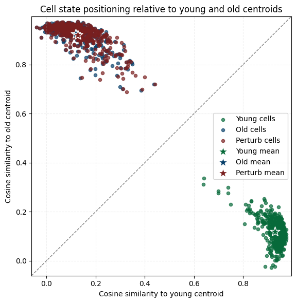
# all cell plot
plot_cosine_to_centroids_with_perturb(
    adata_ori=adata_ori,
    adata_perturb=adata_perturb_final,
    slice_young="Hippocampus_Y_2_1",
    slice_old="Hippocampus_O_2_1",
    target_celltype="OL-WM",
    exclude_celltype=False,
    # save_path=os.path.join(f"{out_fig_dir}/target_cell_cell_stat.pdf")
)

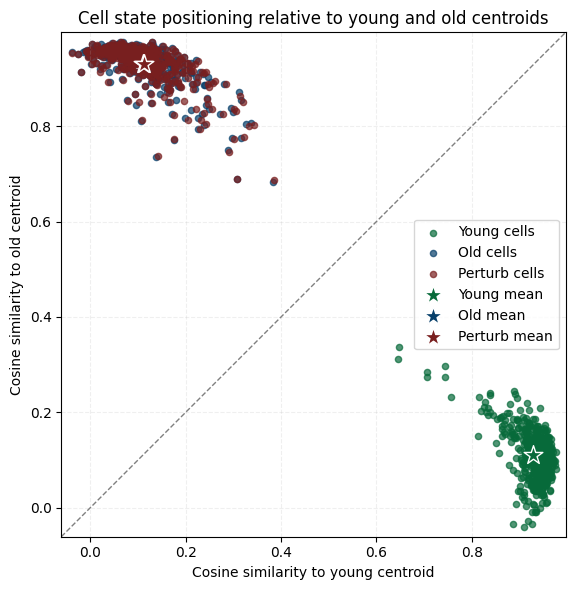
# niche-only
plot_cosine_to_centroids_with_perturb(
    adata_ori=adata_ori,
    adata_perturb=adata_perturb_final,
    slice_young="Hippocampus_Y_2_1",
    slice_old="Hippocampus_O_2_1",
    target_celltype="OL-WM",
    exclude_celltype=True,
    # save_path=os.path.join(f"{out_fig_dir}/niche_cell_cell_stat.pdf")
)

cosine_before_niche, cosine_after_niche = sim_ko_meg3_niche["cosine"]
euclid_before_niche, euclid_after_niche = sim_ko_meg3_niche["euclidean"]
emd_before_niche, emd_after_niche = sim_ko_meg3_niche["emd"]
mmd_before_niche, mmd_after_niche = sim_ko_meg3_niche["mmd"]

print("Niche cosine similarity: before KO = {:.4f}, after KO = {:.4f}".format(cosine_before_niche, cosine_after_niche))
print("Niche Euclidean distance: before KO = {:.4f}, after KO = {:.4f}".format(euclid_before_niche, euclid_after_niche))
print("Niche Wasserstein distance (EMD): before KO = {:.4f}, after KO = {:.4f}".format(emd_before_niche, emd_after_niche))
print("Niche MMD: before KO = {:.4f}, after KO = {:.4f}".format(mmd_before_niche, mmd_after_niche))

Niche cosine similarity: before KO = 0.1120, after KO = 0.1143
Niche Euclidean distance: before KO = 13.0246, after KO = 12.9961
Niche Wasserstein distance (EMD): before KO = 0.3707, after KO = 0.3694
Niche MMD: before KO = 0.0050, after KO = 0.0050