Cell-driven Niche Perturbation (CNP) Replacement Simulation

This tutorial introduces the Cell-driven Niche Perturbation (CNP) framework for probing how targeted cellular perturbations reshape spatial microenvironments in the aging hippocampus.

We use mouse Stereo-seq data from Ma et al., Cell (2024) to demonstrate how cell-level perturbations can causally link cellular identity to niche organization during aging.

⸻

Dataset

Study Spatial transcriptomic landscape unveils immunoglobulin-associated senescence as a hallmark of aging Ma, Shuai et al., Cell, 2024

The dataset captures spatial gene expression patterns in the hippocampus of young (2-month-old) and aged (25-month-old) mice.

⸻

Regions of Interest (ROIs)

Selected hippocampal ROIs from young and aged mice are used as localized spatial contexts to analyze niche-level responses to perturbation.

⸻

CNP Perturbation Modes

1. Cell Replacement

Aged cells within a target niche are replaced by their young counterparts, partially overwriting the aged tissue context. This mode evaluates how rejuvenated cellular identities reshape surrounding microenvironments.

2. Cell Injection

Young cells are introduced into aged ROIs without removing native aged cells. This mode isolates how rejuvenating cues propagate through an intact aged structural substrate.

⸻

Evaluation

For both perturbation modes, we assess: • Spatial remodeling within ROIs • Cell- and niche-level embedding similarity to the young reference • Microenvironmental responses across major cell types

⸻

import os
import torch
import numpy as np
import pandas as pd
import scanpy as sc
import gseapy as gp
import anndata as ad
import seaborn as sns
from typing import Optional
from pathlib import Path
import matplotlib.pyplot as plt
from matplotlib.patches import Rectangle
import matplotlib.colors as mcolors
from matplotlib.colors import LinearSegmentedColormap
import sys
sys.path.append("/inspire/ssd/project/sais-lifescience/public/workspace/yangyiwen/Brainbeacon_v2/BrainBeacon/")
from brainbeacon.pipeline.cell_embedding import run_bbcellformer_pipeline
from brainbeacon.pipeline.perturbation import inject_cells_theory, inject_cells_into_niche, plot_cosine_to_centroids_non_target, analyze_embedding_similarity_change_similarity_niche
from brainbeacon.pipeline.perturbation import analyze_embedding_similarity_change, analyze_gene_reconstruction_change, compute_delta_cosine
from brainbeacon.utils import set_seed
import brainbeacon.configs.config as cfg
from brainbeacon.configs.config_train import config_train as cfg_train
from brainbeacon.utils import compute_density_token, compute_deviation_bin_rapid_v2
from brainbeacon.utils import convert_spatial_to_um, platform_radius_map
import logging
logging.basicConfig(
    level=logging.INFO,  # 或 level=logging.DEBUG
    format='%(asctime)s %(levelname)s %(message)s'
)

import warnings
plt.rcParams["pdf.fonttype"] = 42
warnings.filterwarnings("ignore")
set_seed(42)

Device setup

# Set GPU 
os.environ["CUDA_VISIBLE_DEVICES"] = "0"
device = torch.device("cuda" if torch.cuda.is_available() else "cpu")
print(f"Using device: {device}")
if device.type == "cuda":
    print(f"Using GPU: {torch.cuda.get_device_name(torch.cuda.current_device())}")

# Define base paths and dataset info
out_fig_dir = "/inspire/ssd/project/sais-lifescience/public/yangyiwen_global/Brainbeacon/output/virtual_perturbation/fig5_subfig"
os.makedirs(out_fig_dir, exist_ok=True)

Using device: cuda
Using GPU: NVIDIA H800

Paths and dataset config

Example dataset ()

Path to the processed AnnData object used in this tutorial. The processed file (adata_outer_ensembl.h5ad) can be downloaded directly from: https://drive.google.com/file/d/1-z8J8xiRN0qD0preVQr8cAHKQXuScBp2/view?usp=drive_link Alternatively, the original raw Stereo-seq data can be obtained from the CNGBdb STOmics portal: https://db.cngb.org/stomics/datasets/STDS0000247/data

# =============================================================================
# Dataset and Basic Setup
# =============================================================================
dataset_name = "niche2cell_replacement"
specie = "mouse"  # NOTE: keep original variable name for compatibility
assay = "stereo"

# =============================================================================
# Prior Knowledge / Paths
# =============================================================================
# Base directories
BASE_DIR = Path("/inspire/ssd/project/sais-lifescience/public/yangyiwen_global/Brainbeacon/")

# Sync into cfg (assumes cfg / cfg_train already exist in your notebook/runtime)
cfg.DEFAULT_PATHS["BASE_DIR"] = str(BASE_DIR)
cfg.DEFAULT_PATHS["PRETRAIN_DIR"] = "/inspire/ssd/project/sais-lifescience/public/workspace/yangyiwen/Brainbeacon/bb_PriorKnowledge/"
cfg.DEFAULT_PATHS["PRIOR_DIR"] = cfg.DEFAULT_PATHS["PRETRAIN_DIR"]
cfg.DEFAULT_PATHS["GENE_DICT_PATH"] = (
    "/inspire/ssd/project/sais-lifescience/public/workspace/yangyiwen/Brainbeacon/bb_PriorKnowledge/model_h5ad_1211.h5ad"
)

# Input data
# Users may start from the raw data and follow their own preprocessing pipeline if desired.
adata_path = BASE_DIR / "data" / "adata_outer_ensembl.h5ad"  # adata_outer_ensembl / adata_inner_ensembl
gene_dict_path = Path(cfg.DEFAULT_PATHS["GENE_DICT_PATH"])
gene_mean_path = Path(
    "/inspire/ssd/project/sais-lifescience/public/yangyiwen_global/Brainbeacon/bb_PriorKnowledge/stereo-seq_gene_nonzero_means_metacell_2.npy"
)

# ESM embedding path
cfg_train["esm_embedding_path"] = (
    "/inspire/ssd/project/sais-lifescience/public/workspace/yangyiwen/Brainbeacon/bb_PriorKnowledge/esm2_embeddings_d5120.pt"
)

# Basic sanity checks (fail fast)
assert adata_path.exists(), f"adata_path not found: {adata_path}"
assert gene_dict_path.exists(), f"gene_dict_path not found: {gene_dict_path}"
assert gene_mean_path.exists(), f"gene_mean_path not found: {gene_mean_path}"
assert Path(cfg_train["esm_embedding_path"]).exists(), f"esm_embedding_path not found: {cfg_train['esm_embedding_path']}"

# =============================================================================
# Pretrained Checkpoints
# =============================================================================
pretrain_dir = BASE_DIR / "pretrained"

bb_ckpt_name = "epoch_0_setp_800000.pt"
cellformer_ckpt_name = "cellformer_epoch99.pt"  # trained on all ma2024aging data
# cellformer_ckpt_name = "cellformer.ckpt"      # CellPLM original checkpoint

bb_ckpt_path = Path("/inspire/ssd/project/sais-lifescience/public/yangyiwen_global/Brainbeacon/bb_PriorKnowledge/epoch_0_step_800000.pt")
cellplm_ckpt_path = Path("/inspire/ssd/project/sais-lifescience/public/yangyiwen_global/Brainbeacon/bb_PriorKnowledge/cellformer_epoch99.pt")

assert bb_ckpt_path.exists(), f"bb_ckpt_path not found: {bb_ckpt_path}"
assert cellplm_ckpt_path.exists(), f"cellplm_ckpt_path not found: {cellplm_ckpt_path}"

# =============================================================================
# Output Naming
# =============================================================================
cd_weight = 0.02
use_hvg = True
n_hvg = 5000

bb_ckpt_tag = bb_ckpt_name.replace(".pt", "").replace(".ckpt", "")
if use_hvg:
    method_name = f"bbcellformer_{bb_ckpt_tag}_hvg{n_hvg}_cd{cd_weight}"
else:
    method_name = f"bbcellformer_{bb_ckpt_tag}_cd{cd_weight}"

output_dir = BASE_DIR / "downstream_tasks" / "virtual_perturbation" / "outputs" / dataset_name / method_name
output_dir.mkdir(parents=True, exist_ok=True)

# =============================================================================
# Load Data and (Optionally) Select Slices
# =============================================================================
full_adata = sc.read_h5ad(str(adata_path))

selected_slices = ["Hippocampus_Y_2_1", "Hippocampus_O_2_1"]

# NOTE: Uncomment if you want to restrict to selected slices
# adata = full_adata[full_adata.obs["slice"].isin(selected_slices)].copy()
adata = full_adata.copy()

# =============================================================================
# Derive Labels
# =============================================================================
def infer_cell_label(slice_name: str) -> Optional[str]:
    """Infer 'Young' / 'Old' from slice naming convention."""
    if slice_name.startswith("Hippocampus_Y"):
        return "Young"
    if slice_name.startswith("Hippocampus_O"):
        return "Old"
    return None  # Unknown slice pattern

# Apply label + batch
adata.obs["cell_label"] = adata.obs["slice"].astype(str).map(infer_cell_label)
adata.obs["batch"] = adata.obs["slice"]

# Enforce categorical type (keeps only 'Young' and 'Old' as known categories)
adata.obs["cell_label"] = pd.Categorical(adata.obs["cell_label"], categories=["Young", "Old"])

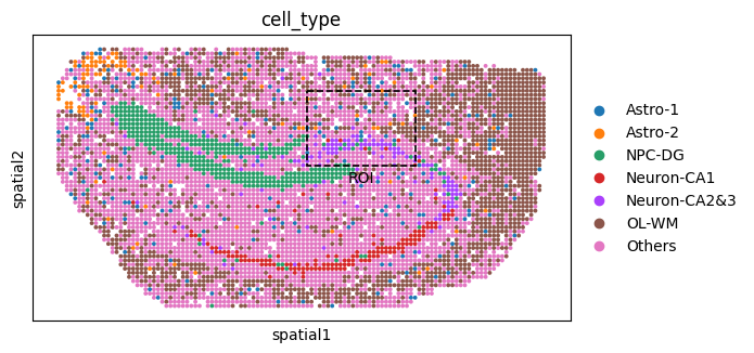
Set ROI

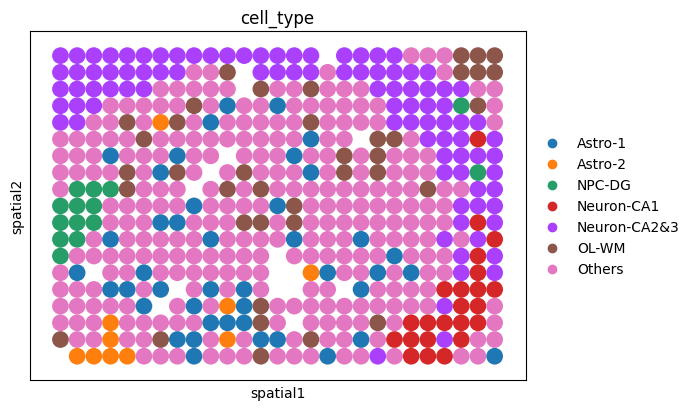
Next, we select regions of interest (ROIs) to further investigate how the perturbation reshapes local cellular niches after gene perturbation. These ROIs enable a focused analysis of spatial and niche-level changes induced by the perturbation.

ol_cells = adata[adata.obs["slice"] == "Hippocampus_O_2_1"].copy()
ol_roi = ol_cells[
    (ol_cells.obsm["spatial"][:, 0] > 60) &    
    (ol_cells.obsm["spatial"][:, 1] > 10) &    
    (ol_cells.obsm["spatial"][:, 0] < 88) &      
    (ol_cells.obsm["spatial"][:, 1] < 30)
].copy()
print(ol_roi)
ol_cells.obs["cell_type"] = ol_cells.obs["cell_type"].astype("category")
categories = ol_cells.obs["cell_type"].cat.categories
ol_roi.obs["cell_type"] = pd.Categorical(
    ol_roi.obs["cell_type"], categories=categories, ordered=True
)

ol_cells.uns["cell_type_colors"] = ol_cells.uns.get(
    "cell_type_colors", sc.pl.palettes.default_20[:len(categories)]
)
ol_roi.uns["cell_type_colors"] = ol_cells.uns["cell_type_colors"]

roi_coords = ol_roi.obsm["spatial"]
xmin, xmax = roi_coords[:, 0].min(), roi_coords[:, 0].max()
ymin, ymax = roi_coords[:, 1].min(), roi_coords[:, 1].max()
xcenter, ycenter = (xmin + xmax) / 2, (ymin + ymax) / 2
os.makedirs(out_fig_dir, exist_ok=True)

fig_ol = sc.pl.spatial(
    ol_cells, color="cell_type", spot_size=1, show=False, return_fig=True
)
ax_ol = fig_ol.axes[0]
rect = Rectangle(
    (xmin, ymin), xmax - xmin, ymax - ymin,
    linewidth=1.2, edgecolor='black', facecolor='none', linestyle='--'
)
ax_ol.add_patch(rect)

ax_ol.text(
    xcenter, ymax + 5, "ROI",
    color='black', fontsize=10, ha='center', va='bottom'
)
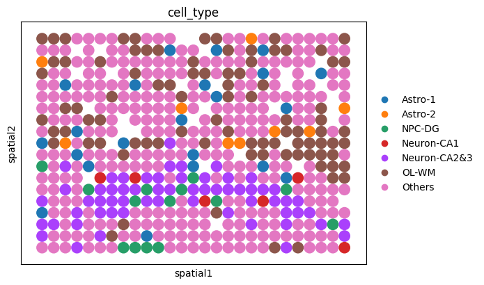
fig_roi = sc.pl.spatial(
    ol_roi, color="cell_type", spot_size=1, show=False, return_fig=True
)

AnnData object with n_obs × n_vars = 481 × 20318
    obs: 'x', 'y', 'cell_type', 'n_genes_by_counts', 'log1p_n_genes_by_counts', 'total_counts', 'log1p_total_counts', 'pct_counts_in_top_50_genes', 'pct_counts_in_top_100_genes', 'pct_counts_in_top_200_genes', 'pct_counts_in_top_500_genes', 'total_counts_mito', 'log1p_total_counts_mito', 'pct_counts_mito', 'clusters', 'cell_label', 'slice', 'species', 'age_group', 'batch'
    var: 'gene_symbol', 'ensembl', 'human_symbol', 'human_ensembl'
    obsm: 'X_pca', 'X_umap', 'spatial'
    layers: 'lognorm', 'raw_count'

# === Matplotlib settings (ensure editable text in PDF/SVG) ===
warnings.filterwarnings("ignore")
logging.getLogger('matplotlib.font_manager').disabled = True

plt.rcParams['pdf.fonttype'] = 42
plt.rcParams['ps.fonttype']  = 42
plt.rcParams['svg.fonttype'] = 'none'
plt.rcParams['font.sans-serif'] = ['Arial']
plt.rcParams['font.family'] = 'sans-serif'

# === Ensure output directory ===
os.makedirs(out_fig_dir, exist_ok=True)

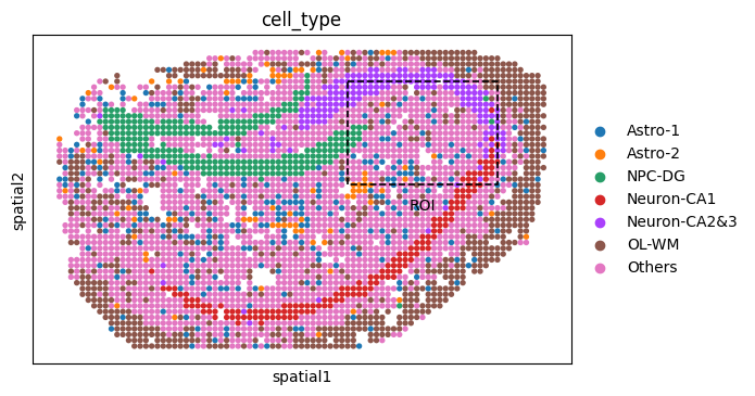
# === Step 1: subset slice ===
adata_Y = adata[adata.obs["slice"] == "Hippocampus_Y_2_1"].copy()

# === Step 2: coordinates ===
x = adata_Y.obsm["spatial"][:, 0]
y = adata_Y.obsm["spatial"][:, 1]
print(f"x: {x.min():.1f} ~ {x.max():.1f}, y: {y.min():.1f} ~ {y.max():.1f}")

# === Step 3: ROI bounds (x in (60, 88), y in (10, 30)) ===
roi_mask = (x > 50) & (x < 78) & (y > 5) & (y < 25)
y_roi = adata_Y[roi_mask].copy()
print(f"ROI cells: {y_roi.n_obs}")

# === Step 4: sync categories & colors ===
adata_Y.obs["cell_type"] = adata_Y.obs["cell_type"].astype("category")
cats = adata_Y.obs["cell_type"].cat.categories
y_roi.obs["cell_type"] = pd.Categorical(y_roi.obs["cell_type"], categories=cats, ordered=True)

adata_Y.uns["cell_type_colors"] = adata_Y.uns.get(
    "cell_type_colors", sc.pl.palettes.default_20[:len(cats)]
)
y_roi.uns["cell_type_colors"] = adata_Y.uns["cell_type_colors"]

# === Step 5a: full view with ROI box ===
fig1 = sc.pl.spatial(adata_Y, color="cell_type", spot_size=1, show=False, return_fig=True)

# Add dashed ROI box
roi_xy = y_roi.obsm["spatial"]
xmin, xmax = roi_xy[:, 0].min(), roi_xy[:, 0].max()
ymin, ymax = roi_xy[:, 1].min(), roi_xy[:, 1].max()
xcenter, ycenter = (xmin + xmax) / 2, (ymin + ymax) / 2

ax = fig1.axes[0]
rect = Rectangle((xmin, ymin), xmax - xmin, ymax - ymin,
                 linewidth=1.2, edgecolor='black', facecolor='none', linestyle='--')
ax.add_patch(rect)
ax.text(xcenter, ymax + 5, "ROI", color='black', fontsize=10, ha='center', va='bottom')
# === Step 5b: ROI-only ===
fig2 = sc.pl.spatial(y_roi, color="cell_type", spot_size=1, show=False, return_fig=True)

x: 1.0 ~ 85.0, y: 1.0 ~ 52.0
ROI cells: 495

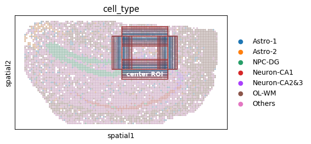
fig_ol = sc.pl.spatial(
    ol_cells,
    color="cell_type",
    spot_size=1,
    show=False,
    return_fig=True
)
ax_ol = fig_ol.axes[0]

for c in ax_ol.collections:
    facecolors = c.get_facecolor()
    # Gray
    gray = np.array([0.5, 0.5, 0.5, 1.0])
    mixed = 0.5 * facecolors + 0.5 * gray
    c.set_facecolor(mixed)
    c.set_alpha(0.5)   

# === ROI ===
ol_base_x, ol_base_y = (60, 88), (10, 30)
shifts = [(0, 0), (1, 0), (-1, 0), (0, 1), (0, -1),
           (2, 0), (-2, 0), (0, 2), (0, -2),
           (3, 0), (-3, 0), (0, 3), (0, -3),
           (4, 0), (-4, 0), (0, 4), (0, -4),
           (5, 0), (-5, 0), (0, 5), (0, -5),
           (6, 0), (-6, 0), (0, 6), (0, -6)]

import matplotlib.colors as mcolors
start_color = "#145583" 
end_color   = "#A13939" 
cmap = mcolors.LinearSegmentedColormap.from_list("blue_red", [start_color, end_color])
colors = [cmap(i / (len(shifts)-1)) for i in range(len(shifts))]

# ===  ROI box===
for i, (dx, dy) in enumerate(shifts):
    xmin, xmax = ol_base_x[0] + dx, ol_base_x[1] + dx
    ymin, ymax = ol_base_y[0] + dy, ol_base_y[1] + dy
    rect = Rectangle(
        (xmin, ymin),
        xmax - xmin,
        ymax - ymin,
        linewidth=1.4,
        edgecolor=colors[i],
        facecolor='none',
        linestyle='-',
        alpha=0.95,
    )
    ax_ol.add_patch(rect)

# ===  ROI anno ===
ax_ol.text(
    np.mean(ol_base_x),
    ol_base_y[1] + 5,
    "center ROI",
    color='white',
    fontsize=9,
    weight='bold',
    ha='center',
    va='bottom'
)

plt.tight_layout()
# plt.savefig(f"{out_fig_dir}/ol_cells_with_multiple_roi_boxes.pdf", bbox_inches="tight")
plt.show()

ol_roi.obs["brain_region"] = ol_roi.obs["slice"]
ol_roi.obs["brain_region_main"] = ol_roi.obs["slice"]
ol_roi.obsm["spatial"] = ol_roi.obsm["spatial"].astype(np.float32)
ol_roi = compute_deviation_bin_rapid_v2(ol_roi)
ol_roi = convert_spatial_to_um(ol_roi, "STEREO")
radius = platform_radius_map.get("STEREO_bin", 8)
ol_roi, _ = compute_density_token(ol_roi, radius)

y_roi.obs["brain_region"] = y_roi.obs["slice"]
y_roi.obs["brain_region_main"] = y_roi.obs["slice"]
y_roi.obsm["spatial"] = y_roi.obsm["spatial"].astype(np.float32)
y_roi = compute_deviation_bin_rapid_v2(y_roi)
y_roi = convert_spatial_to_um(y_roi, "STEREO")
radius = platform_radius_map.get("STEREO_bin", 8)
y_roi, _ = compute_density_token(y_roi, radius)

adata_fov_OL = ad.concat([ol_roi, y_roi], join="outer")
adata_fov_OL.var = adata.var.loc[adata_fov_OL.var_names].copy()
output_prefix_ori = "original"
adata_fov_OL.obs["split"] = "train"
os.makedirs(output_dir, exist_ok=True)
ori_input_adata_path = os.path.join(output_dir, f"{output_prefix_ori}_input.h5ad")
adata_fov_OL.write(ori_input_adata_path)
print(f"Saved selected slices to: {ori_input_adata_path}")

Saved selected slices to: /inspire/ssd/project/sais-lifescience/public/yangyiwen_global/Brainbeacon/downstream_tasks/virtual_perturbation/outputs/niche2cell_replacement/bbcellformer_epoch_0_setp_800000_hvg5000_cd0.02/original_input.h5ad

print(ol_roi)
print(y_roi)
print(adata)
print(adata_fov_OL)

AnnData object with n_obs × n_vars = 481 × 20318
    obs: 'x', 'y', 'cell_type', 'n_genes_by_counts', 'log1p_n_genes_by_counts', 'total_counts', 'log1p_total_counts', 'pct_counts_in_top_50_genes', 'pct_counts_in_top_100_genes', 'pct_counts_in_top_200_genes', 'pct_counts_in_top_500_genes', 'total_counts_mito', 'log1p_total_counts_mito', 'pct_counts_mito', 'clusters', 'cell_label', 'slice', 'species', 'age_group', 'batch', 'brain_region', 'brain_region_main', 'slice_brain_area', 'density_token'
    var: 'gene_symbol', 'ensembl', 'human_symbol', 'human_ensembl'
    uns: 'cell_type_colors'
    obsm: 'X_pca', 'X_umap', 'spatial', 'deviation_bin', 'neighbor_gene_distribution', 'spatial_um'
    layers: 'lognorm', 'raw_count'
AnnData object with n_obs × n_vars = 495 × 20318
    obs: 'x', 'y', 'cell_type', 'n_genes_by_counts', 'log1p_n_genes_by_counts', 'total_counts', 'log1p_total_counts', 'pct_counts_in_top_50_genes', 'pct_counts_in_top_100_genes', 'pct_counts_in_top_200_genes', 'pct_counts_in_top_500_genes', 'total_counts_mito', 'log1p_total_counts_mito', 'pct_counts_mito', 'clusters', 'cell_label', 'slice', 'species', 'age_group', 'batch', 'brain_region', 'brain_region_main', 'slice_brain_area', 'density_token'
    var: 'gene_symbol', 'ensembl', 'human_symbol', 'human_ensembl'
    uns: 'cell_type_colors'
    obsm: 'X_pca', 'X_umap', 'spatial', 'deviation_bin', 'neighbor_gene_distribution', 'spatial_um'
    layers: 'lognorm', 'raw_count'
AnnData object with n_obs × n_vars = 57140 × 20318
    obs: 'x', 'y', 'cell_type', 'n_genes_by_counts', 'log1p_n_genes_by_counts', 'total_counts', 'log1p_total_counts', 'pct_counts_in_top_50_genes', 'pct_counts_in_top_100_genes', 'pct_counts_in_top_200_genes', 'pct_counts_in_top_500_genes', 'total_counts_mito', 'log1p_total_counts_mito', 'pct_counts_mito', 'clusters', 'cell_label', 'slice', 'species', 'age_group', 'batch'
    var: 'gene_symbol', 'ensembl', 'human_symbol', 'human_ensembl'
    obsm: 'X_pca', 'X_umap', 'spatial'
    layers: 'lognorm', 'raw_count'
AnnData object with n_obs × n_vars = 976 × 20318
    obs: 'x', 'y', 'cell_type', 'n_genes_by_counts', 'log1p_n_genes_by_counts', 'total_counts', 'log1p_total_counts', 'pct_counts_in_top_50_genes', 'pct_counts_in_top_100_genes', 'pct_counts_in_top_200_genes', 'pct_counts_in_top_500_genes', 'total_counts_mito', 'log1p_total_counts_mito', 'pct_counts_mito', 'clusters', 'cell_label', 'slice', 'species', 'age_group', 'batch', 'brain_region', 'brain_region_main', 'slice_brain_area', 'density_token', 'split'
    var: 'gene_symbol', 'ensembl', 'human_symbol', 'human_ensembl'
    obsm: 'X_pca', 'X_umap', 'spatial', 'deviation_bin', 'neighbor_gene_distribution', 'spatial_um'
    layers: 'lognorm', 'raw_count'

Run Original Inference

This step constructs the baseline (unperturbed) reference by running inference kon the original data, which serves as the control condition for all subsequent perturbation analyses.

adata_ori = run_bbcellformer_pipeline(
    adata_path=ori_input_adata_path,
    specie=specie,
    assay=assay,
    gene_dict_path=gene_dict_path,
    gene_mean_path=gene_mean_path,
    bb_ckpt_path=bb_ckpt_path,
    cellplm_ckpt_path=cellplm_ckpt_path,
    output_dir=output_dir,
    output_prefix=output_prefix_ori,
    config_train=cfg_train,
    n_hvg=n_hvg,
    cd_weight=cd_weight,
    use_hvg=use_hvg,
    weight_mode="expression",
    use_batch=False,
    use_spatial=True,
    force_tokenize=True,
    do_fit=True,  # recommended to set to True for original reconstruction
    device=device,
    fit_epochs=100,
)
print("Original reconstruction complete. Embeddings and model saved.")
print("adata_ori:", adata_ori)

ori_result_adata_path = os.path.join(output_dir, f"{output_prefix_ori}_result.h5ad")
adata_ori.write(ori_result_adata_path)
print(f"Original result adata saved to: {ori_result_adata_path}")

Forcing re-tokenization: clearing existing .parquet files and token folders...
No existing tokenized files found. Running tokenization...
path to process: /inspire/ssd/project/sais-lifescience/public/yangyiwen_global/Brainbeacon/downstream_tasks/virtual_perturbation/outputs/niche2cell_replacement/bbcellformer_epoch_0_setp_800000_hvg5000_cd0.02/original_input.h5ad
before quality control adata shape: (976, 20318)
After HVG (5000) selection: (976, 5000)
Computing cell density...
compute_density_token time:  0.0038668354352315265 min
Begin processing: /inspire/ssd/project/sais-lifescience/public/yangyiwen_global/Brainbeacon/downstream_tasks/virtual_perturbation/outputs/niche2cell_replacement/bbcellformer_epoch_0_setp_800000_hvg5000_cd0.02/original_bb_token_dir/tokens-0000.parquet
Table shape from parquet = 976
Preprocessing time: 0.12 minutes
Loaded pretrain_model checkpoint: /inspire/ssd/project/sais-lifescience/public/yangyiwen_global/Brainbeacon/bb_PriorKnowledge/epoch_0_step_800000.pt
obs_names and pred_indices are in the same order.
Embeddings saved to /inspire/ssd/project/sais-lifescience/public/yangyiwen_global/Brainbeacon/downstream_tasks/virtual_perturbation/outputs/niche2cell_replacement/bbcellformer_epoch_0_setp_800000_hvg5000_cd0.02/original_bb_embeddings.npz
Time cost:  0.31237366994222004
BB inference complete. Saved to: /inspire/ssd/project/sais-lifescience/public/yangyiwen_global/Brainbeacon/downstream_tasks/virtual_perturbation/outputs/niche2cell_replacement/bbcellformer_epoch_0_setp_800000_hvg5000_cd0.02/original_bb_embeddings.npz
[INFO] Using explicitly provided CellFormer checkpoint: /inspire/ssd/project/sais-lifescience/public/yangyiwen_global/Brainbeacon/bb_PriorKnowledge/cellformer_epoch99.pt
********** gene list size: 92076 **********
********** loading skip parameters: set() **********
After filtering, 20316 genes remain.
Epoch 0 | Train loss: 19754.3462 | Valid loss: 20418.4263
Epoch 1 | Train loss: 17814.4434 | Valid loss: 17169.4941
Epoch 2 | Train loss: 15183.4585 | Valid loss: 13781.2520
Epoch 3 | Train loss: 11961.5400 | Valid loss: 10546.7905
Epoch 4 | Train loss: 9717.5762 | Valid loss: 8113.6162
Epoch 5 | Train loss: 7772.9041 | Valid loss: 7407.3206
Epoch 6 | Train loss: 7313.2432 | Valid loss: 7223.4465
Epoch 7 | Train loss: 7241.3916 | Valid loss: 7218.8459
Epoch 8 | Train loss: 7173.7888 | Valid loss: 7216.5046
Epoch 9 | Train loss: 7202.7556 | Valid loss: 7213.8367
Epoch 10 | Train loss: 7336.0952 | Valid loss: 7210.1489
Epoch 11 | Train loss: 7185.5908 | Valid loss: 7206.6870
Epoch 12 | Train loss: 7419.1924 | Valid loss: 7202.9348
Epoch 13 | Train loss: 7183.8896 | Valid loss: 7198.8628
Epoch 14 | Train loss: 7136.3804 | Valid loss: 7195.8555
Epoch 15 | Train loss: 7220.1282 | Valid loss: 7191.6562
Epoch 16 | Train loss: 7207.6970 | Valid loss: 7188.3438
Epoch 17 | Train loss: 7234.3596 | Valid loss: 7184.7644
Epoch 18 | Train loss: 7086.0078 | Valid loss: 7180.6450
Epoch 19 | Train loss: 7186.0859 | Valid loss: 7176.7720
Epoch 20 | Train loss: 7314.2183 | Valid loss: 7171.2444
Epoch 21 | Train loss: 7039.5352 | Valid loss: 7162.0793
Epoch 22 | Train loss: 7108.5981 | Valid loss: 7162.9985
Epoch 23 | Train loss: 7162.5605 | Valid loss: 7153.5894
Epoch 24 | Train loss: 7172.5879 | Valid loss: 7153.8652
Epoch 25 | Train loss: 7164.2371 | Valid loss: 7147.8079
Epoch 26 | Train loss: 7072.0237 | Valid loss: 7142.3708
Epoch 27 | Train loss: 7235.6038 | Valid loss: 7143.4756
Epoch 28 | Train loss: 7169.2344 | Valid loss: 7139.4495
Epoch 29 | Train loss: 7099.4167 | Valid loss: 7131.1633
Epoch 30 | Train loss: 7199.0378 | Valid loss: 7129.1655
Epoch 31 | Train loss: 7277.7117 | Valid loss: 7124.9893
Epoch 32 | Train loss: 7105.2947 | Valid loss: 7119.7693
Epoch 33 | Train loss: 7005.3721 | Valid loss: 7117.6055
Epoch 34 | Train loss: 7091.3821 | Valid loss: 7112.8389
Epoch 35 | Train loss: 7042.4587 | Valid loss: 7108.1072
Epoch 36 | Train loss: 7141.8374 | Valid loss: 7103.7412
Epoch 37 | Train loss: 7117.8672 | Valid loss: 7099.7349
Epoch 38 | Train loss: 7023.4429 | Valid loss: 7094.4160
Epoch 39 | Train loss: 7052.7529 | Valid loss: 7089.2034
Epoch 40 | Train loss: 7008.0156 | Valid loss: 7084.6860
Epoch 41 | Train loss: 7140.2300 | Valid loss: 7080.0132
Epoch 42 | Train loss: 7011.5356 | Valid loss: 7075.1487
Epoch 43 | Train loss: 7187.6658 | Valid loss: 7070.1191
Epoch 44 | Train loss: 7162.8506 | Valid loss: 7064.9451
Epoch 45 | Train loss: 6939.2012 | Valid loss: 7059.8992
Epoch 46 | Train loss: 6983.5208 | Valid loss: 7054.8860
Epoch 47 | Train loss: 7025.1587 | Valid loss: 7049.5667
Epoch 48 | Train loss: 7034.9082 | Valid loss: 7044.4058
Epoch 49 | Train loss: 7024.4331 | Valid loss: 7039.7097
Epoch 50 | Train loss: 6972.8816 | Valid loss: 7034.4268
Epoch 51 | Train loss: 7055.8447 | Valid loss: 7029.2246
Epoch 52 | Train loss: 7000.6719 | Valid loss: 7024.8030
Epoch 53 | Train loss: 7098.1392 | Valid loss: 7020.6677
Epoch 54 | Train loss: 6944.7014 | Valid loss: 7016.8149
Epoch 55 | Train loss: 6951.4971 | Valid loss: 7012.1958
Epoch 56 | Train loss: 7022.1548 | Valid loss: 7006.7651
Epoch 57 | Train loss: 7018.0371 | Valid loss: 7002.4963
Epoch 58 | Train loss: 7031.2852 | Valid loss: 6998.7092
Epoch 59 | Train loss: 6929.1497 | Valid loss: 6995.4094
Epoch 60 | Train loss: 7036.0046 | Valid loss: 6991.7349
Epoch 61 | Train loss: 6976.5562 | Valid loss: 6987.4307
Epoch 62 | Train loss: 6927.7271 | Valid loss: 6983.2922
Epoch 63 | Train loss: 7000.6475 | Valid loss: 6979.1929
Epoch 64 | Train loss: 7093.4644 | Valid loss: 6975.1660
Epoch 65 | Train loss: 6926.8337 | Valid loss: 6971.0662
Epoch 66 | Train loss: 6851.7664 | Valid loss: 6966.5933
Epoch 67 | Train loss: 7034.8625 | Valid loss: 6962.4028
Epoch 68 | Train loss: 6878.9407 | Valid loss: 6958.4116
Epoch 69 | Train loss: 6999.4861 | Valid loss: 6954.3601
Epoch 70 | Train loss: 7005.4026 | Valid loss: 6950.0229
Epoch 71 | Train loss: 6938.2839 | Valid loss: 6945.4683
Epoch 72 | Train loss: 6919.0798 | Valid loss: 6941.2195
Epoch 73 | Train loss: 6975.8445 | Valid loss: 6937.4939
Epoch 74 | Train loss: 6994.0798 | Valid loss: 6933.9502
Epoch 75 | Train loss: 7068.9517 | Valid loss: 6930.2771
Epoch 76 | Train loss: 6771.8110 | Valid loss: 6926.0325
Epoch 77 | Train loss: 7116.1509 | Valid loss: 6922.0166
Epoch 78 | Train loss: 6822.9250 | Valid loss: 6918.2007
Epoch 79 | Train loss: 6880.4580 | Valid loss: 6914.6807
Epoch 80 | Train loss: 6768.1404 | Valid loss: 6911.0068
Epoch 81 | Train loss: 6660.9297 | Valid loss: 6906.6199
Epoch 82 | Train loss: 6833.1191 | Valid loss: 6902.5620
Epoch 83 | Train loss: 6880.1580 | Valid loss: 6898.6567
Epoch 84 | Train loss: 6931.6531 | Valid loss: 6895.2039
Epoch 85 | Train loss: 6855.9238 | Valid loss: 6891.3103
Epoch 86 | Train loss: 6990.7883 | Valid loss: 6887.4758
Epoch 87 | Train loss: 6835.4873 | Valid loss: 6883.1985
Epoch 88 | Train loss: 6870.0300 | Valid loss: 6879.4187
Epoch 89 | Train loss: 6879.7190 | Valid loss: 6875.8972
Epoch 90 | Train loss: 6798.6077 | Valid loss: 6872.0786
Epoch 91 | Train loss: 6907.3708 | Valid loss: 6868.3650
Epoch 92 | Train loss: 6903.1123 | Valid loss: 6864.8435
Epoch 93 | Train loss: 6883.6060 | Valid loss: 6861.2314
Epoch 94 | Train loss: 6739.6294 | Valid loss: 6857.4692
Epoch 95 | Train loss: 6816.6841 | Valid loss: 6853.9160
Epoch 96 | Train loss: 6855.8743 | Valid loss: 6850.5432
Epoch 97 | Train loss: 6965.2151 | Valid loss: 6847.2788
Epoch 98 | Train loss: 6803.6355 | Valid loss: 6843.8608
Epoch 99 | Train loss: 6832.2544 | Valid loss: 6840.0640
After filtering, 20316 genes remain.
Model saved to /inspire/ssd/project/sais-lifescience/public/yangyiwen_global/Brainbeacon/downstream_tasks/virtual_perturbation/outputs/niche2cell_replacement/bbcellformer_epoch_0_setp_800000_hvg5000_cd0.02/original_cellformer.pt
Embeddings saved to /inspire/ssd/project/sais-lifescience/public/yangyiwen_global/Brainbeacon/downstream_tasks/virtual_perturbation/outputs/niche2cell_replacement/bbcellformer_epoch_0_setp_800000_hvg5000_cd0.02/original_embeddings.npz
Original reconstruction complete. Embeddings and model saved.
adata_ori: AnnData object with n_obs × n_vars = 976 × 20316
    obs: 'x', 'y', 'cell_type', 'n_genes_by_counts', 'log1p_n_genes_by_counts', 'total_counts', 'log1p_total_counts', 'pct_counts_in_top_50_genes', 'pct_counts_in_top_100_genes', 'pct_counts_in_top_200_genes', 'pct_counts_in_top_500_genes', 'total_counts_mito', 'log1p_total_counts_mito', 'pct_counts_mito', 'clusters', 'cell_label', 'slice', 'species', 'age_group', 'batch', 'brain_region', 'brain_region_main', 'slice_brain_area', 'density_token', 'split', 'platform', 'valid_split', 'x_FOV_px', 'y_FOV_px'
    var: 'gene_symbol', 'ensembl', 'human_symbol', 'human_ensembl'
    obsm: 'X_pca', 'X_umap', 'deviation_bin', 'neighbor_gene_distribution', 'spatial', 'spatial_um', 'bb_emb', 'X_emb', 'X_pred'
    layers: 'lognorm', 'raw_count'
Original result adata saved to: /inspire/ssd/project/sais-lifescience/public/yangyiwen_global/Brainbeacon/downstream_tasks/virtual_perturbation/outputs/niche2cell_replacement/bbcellformer_epoch_0_setp_800000_hvg5000_cd0.02/original_result.h5ad

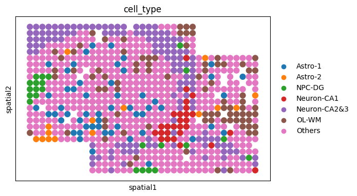
CNP Perturbation (Replacement): Young NPC-DG cells replace aged NPC-DG in situ

This block implements the “replacement” mode in the Cell-driven Niche Perturbation (CNP) framework.

Using NPC-DG as an example, aged NPC-DG cells in the old hippocampal slice are in situ replaced by their young counterparts sampled from the young slice.

This operation preserves the surrounding aged tissue context while overwriting the cellular identity of the target cell type, enabling evaluation of how rejuvenated cells remodel local niches.

Downstream analyses quantify niche-level changes using four metrics: cosine similarity, Euclidean distance, Wasserstein distance (EMD), and MMD.

celltype = "NPC-DG"
SLICE_YOUNG = "Hippocampus_Y_2_1"
SLICE_OLD = "Hippocampus_O_2_1"
old_slice  = adata_fov_OL[adata_fov_OL.obs["slice"] == SLICE_OLD]
young_pool = adata_fov_OL[adata_fov_OL.obs["slice"] == SLICE_YOUNG]

perturbed_adata = inject_cells_theory(
    target_adata = old_slice,
    donor_adata  = young_pool,
    celltype     = celltype,
    spatial_key  = "spatial",
    random_state = 4
)
pert_input = ad.concat(
    [perturbed_adata, adata_fov_OL[adata_fov_OL.obs["slice"] == "Hippocampus_Y_2_1"]],
    join="outer"
)
output_prefix_perturb = "inject_young_NPC-DG_to_old"
perturb_input_adata_path = os.path.join(output_dir, f"{output_prefix_perturb}_input.h5ad")
pert_input.write(perturb_input_adata_path)
print(f"Injected input adata saved to: {perturb_input_adata_path}")

# ========== 8. Run Perturbation Inference ==========
cellplm_ckpt_path = os.path.join(output_dir, f"{output_prefix_ori}_cellformer.pt")
adata_perturb = run_bbcellformer_pipeline(
    adata_path=perturb_input_adata_path,
    specie=specie,
    assay=assay,
    gene_dict_path=gene_dict_path,
    gene_mean_path=gene_mean_path,
    bb_ckpt_path=bb_ckpt_path,
    cellplm_ckpt_path=cellplm_ckpt_path,
    output_dir=output_dir,
    output_prefix=output_prefix_perturb,
    config_train=cfg_train,
    n_hvg=n_hvg,
    cd_weight=cd_weight,
    use_hvg=use_hvg,
    use_batch=False,
    use_spatial=True,
    weight_mode="expression",
    force_tokenize=True,
    do_fit=False,
    fit_epochs=10,
    device=device
)
print("Perturbation reconstruction complete. Embeddings and model saved.")
print("adata_perturb:", adata_perturb)

perturb_result_adata_path = os.path.join(output_dir, f"{output_prefix_perturb}_result.h5ad")
adata_perturb.write(perturb_result_adata_path)
print(f"Perturbation result adat2a saved to: {perturb_result_adata_path}")
adata_injected_celltype = adata_perturb[adata_perturb.obs["injected"].notna()].copy()
adata_injected_celltype.obs["injected"] = adata_injected_celltype.obs["injected"].astype(bool)
adata_perturb_sub = adata_injected_celltype[~adata_injected_celltype.obs["injected"]].copy()

Injected input adata saved to: /inspire/ssd/project/sais-lifescience/public/yangyiwen_global/Brainbeacon/downstream_tasks/virtual_perturbation/outputs/niche2cell_replacement/bbcellformer_epoch_0_setp_800000_hvg5000_cd0.02/inject_young_NPC-DG_to_old_input.h5ad
Forcing re-tokenization: clearing existing .parquet files and token folders...
No existing tokenized files found. Running tokenization...
path to process: /inspire/ssd/project/sais-lifescience/public/yangyiwen_global/Brainbeacon/downstream_tasks/virtual_perturbation/outputs/niche2cell_replacement/bbcellformer_epoch_0_setp_800000_hvg5000_cd0.02/inject_young_NPC-DG_to_old_input.h5ad
before quality control adata shape: (976, 20318)
After HVG (5000) selection: (976, 5000)
Computing cell density...
compute_density_token time:  0.0039066950480143225 min
Begin processing: /inspire/ssd/project/sais-lifescience/public/yangyiwen_global/Brainbeacon/downstream_tasks/virtual_perturbation/outputs/niche2cell_replacement/bbcellformer_epoch_0_setp_800000_hvg5000_cd0.02/inject_young_NPC-DG_to_old_bb_token_dir/tokens-0000.parquet
Table shape from parquet = 976
Preprocessing time: 0.04 minutes
Loaded pretrain_model checkpoint: /inspire/ssd/project/sais-lifescience/public/yangyiwen_global/Brainbeacon/bb_PriorKnowledge/epoch_0_step_800000.pt
obs_names and pred_indices are in the same order.
Embeddings saved to /inspire/ssd/project/sais-lifescience/public/yangyiwen_global/Brainbeacon/downstream_tasks/virtual_perturbation/outputs/niche2cell_replacement/bbcellformer_epoch_0_setp_800000_hvg5000_cd0.02/inject_young_NPC-DG_to_old_bb_embeddings.npz
Time cost:  0.28074302673339846
BB inference complete. Saved to: /inspire/ssd/project/sais-lifescience/public/yangyiwen_global/Brainbeacon/downstream_tasks/virtual_perturbation/outputs/niche2cell_replacement/bbcellformer_epoch_0_setp_800000_hvg5000_cd0.02/inject_young_NPC-DG_to_old_bb_embeddings.npz
[INFO] Using explicitly provided CellFormer checkpoint: /inspire/ssd/project/sais-lifescience/public/yangyiwen_global/Brainbeacon/downstream_tasks/virtual_perturbation/outputs/niche2cell_replacement/bbcellformer_epoch_0_setp_800000_hvg5000_cd0.02/original_cellformer.pt
********** gene list size: 92076 **********
********** loading skip parameters: set() **********
After filtering, 20316 genes remain.
Model saved to /inspire/ssd/project/sais-lifescience/public/yangyiwen_global/Brainbeacon/downstream_tasks/virtual_perturbation/outputs/niche2cell_replacement/bbcellformer_epoch_0_setp_800000_hvg5000_cd0.02/inject_young_NPC-DG_to_old_cellformer.pt
Embeddings saved to /inspire/ssd/project/sais-lifescience/public/yangyiwen_global/Brainbeacon/downstream_tasks/virtual_perturbation/outputs/niche2cell_replacement/bbcellformer_epoch_0_setp_800000_hvg5000_cd0.02/inject_young_NPC-DG_to_old_embeddings.npz
Perturbation reconstruction complete. Embeddings and model saved.
adata_perturb: AnnData object with n_obs × n_vars = 976 × 20316
    obs: 'x', 'y', 'cell_type', 'n_genes_by_counts', 'log1p_n_genes_by_counts', 'total_counts', 'log1p_total_counts', 'pct_counts_in_top_50_genes', 'pct_counts_in_top_100_genes', 'pct_counts_in_top_200_genes', 'pct_counts_in_top_500_genes', 'total_counts_mito', 'log1p_total_counts_mito', 'pct_counts_mito', 'clusters', 'cell_label', 'slice', 'species', 'age_group', 'batch', 'brain_region', 'brain_region_main', 'slice_brain_area', 'density_token', 'split', 'injected', 'injected_celltype', 'platform', 'valid_split', 'x_FOV_px', 'y_FOV_px'
    obsm: 'X_pca', 'X_umap', 'deviation_bin', 'neighbor_gene_distribution', 'spatial', 'spatial_um', 'bb_emb', 'X_emb', 'X_pred'
    layers: 'lognorm', 'raw_count'
Perturbation result adat2a saved to: /inspire/ssd/project/sais-lifescience/public/yangyiwen_global/Brainbeacon/downstream_tasks/virtual_perturbation/outputs/niche2cell_replacement/bbcellformer_epoch_0_setp_800000_hvg5000_cd0.02/inject_young_NPC-DG_to_old_result.h5ad

Niche-level similarity analysis after CNP replacement

We quantify how the replacement perturbation shifts the aged niche toward the young reference state for the target cell type (NPC-DG).

replacement_niche_result = analyze_embedding_similarity_change_similarity_niche(
    adata_ori_result=adata_ori,
    adata_perturb_result=adata_perturb_sub,
    target_slice_young=SLICE_YOUNG,
    target_slice_old=SLICE_OLD,
    target_celltype="NPC-DG",
    embedding_key="X_emb",
)

# Unpack similarity metrics (before vs after replacement)
cosine_before_rep, cosine_after_rep = replacement_niche_result["cosine"]
euclid_before_rep, euclid_after_rep = replacement_niche_result["euclidean"]
emd_before_rep, emd_after_rep = replacement_niche_result["emd"]
mmd_before_rep, mmd_after_rep = replacement_niche_result["mmd"]

print("CNP replacement (NPC-DG) — niche similarity to young reference:")
print("  Cosine similarity        : before = {:.4f}, after = {:.4f}".format(cosine_before_rep, cosine_after_rep))
print("  Euclidean distance       : before = {:.4f}, after = {:.4f}".format(euclid_before_rep, euclid_after_rep))
print("  Wasserstein distance (EMD): before = {:.4f}, after = {:.4f}".format(emd_before_rep, emd_after_rep))
print("  MMD                      : before = {:.4f}, after = {:.4f}".format(mmd_before_rep, mmd_after_rep))

CNP replacement (NPC-DG) — niche similarity to young reference:
  Cosine similarity        : before = 0.1176, after = 0.1345
  Euclidean distance       : before = 12.8969, after = 12.7644
  Wasserstein distance (EMD): before = 0.3651, after = 0.3609
  MMD                      : before = 0.0043, after = 0.0043

sc.pl.spatial(adata_perturb, color="cell_type", spot_size=1)

adata_injected_celltype = adata_perturb[adata_perturb.obs["injected"].notna()].copy()
adata_injected_celltype.obs["injected"] = adata_injected_celltype.obs["injected"].astype(bool)
adata_perturb_sub = adata_injected_celltype[~adata_injected_celltype.obs["injected"]].copy()
SLICE_OLD   = "Hippocampus_O_2_1"
SLICE_YOUNG = "Hippocampus_Y_2_1"

adata_perturb.obs["injected"]

61_11-Hippocampus_O_2_1    False
61_12-Hippocampus_O_2_1    False
61_13-Hippocampus_O_2_1    False
61_14-Hippocampus_O_2_1    False
61_15-Hippocampus_O_2_1    False
                           ...  
77_24-Hippocampus_Y_2_1     <NA>
77_6-Hippocampus_Y_2_1      <NA>
77_7-Hippocampus_Y_2_1      <NA>
77_8-Hippocampus_Y_2_1      <NA>
77_9-Hippocampus_Y_2_1      <NA>
Name: injected, Length: 976, dtype: boolean

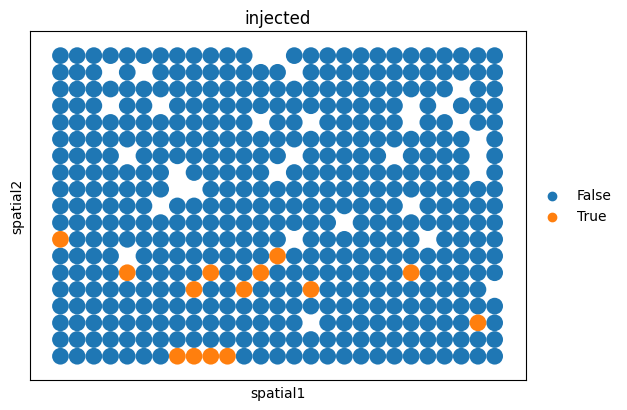
sc.pl.spatial(adata_injected_celltype, color="injected", spot_size=1)

adata_perturb_sub.obs["injected"]

61_11-Hippocampus_O_2_1    False
61_12-Hippocampus_O_2_1    False
61_13-Hippocampus_O_2_1    False
61_14-Hippocampus_O_2_1    False
61_15-Hippocampus_O_2_1    False
                           ...  
87_24-Hippocampus_O_2_1    False
87_26-Hippocampus_O_2_1    False
87_27-Hippocampus_O_2_1    False
87_28-Hippocampus_O_2_1    False
87_29-Hippocampus_O_2_1    False
Name: injected, Length: 467, dtype: bool

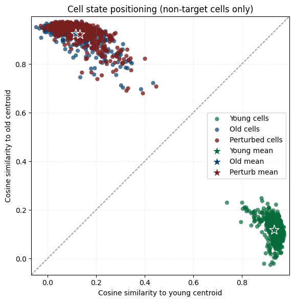
plot_cosine_to_centroids_non_target(
    adata_ori=adata_ori,
    adata_perturb=adata_perturb_sub,
    slice_young=SLICE_YOUNG,
    slice_old=SLICE_OLD, 
    target_cell="NPC-DG",
    emb_key="X_emb",
    # save_path="cosine_scatter_theory.pdf"
)

[INFO] Excluding target cell type: NPC-DG
[INFO] Remaining cells - Young: 481, Old: 467, Perturb: 467

def analyze_inject_gene_reconstruction_change(
    adata_ori_result,
    adata_perturb_result,
    target_cell=None,             # Optional: cell type to exclude from analysis
    target_obs_names=None,
    filter_by=None,
    top_n=100,
    sort_abs=True,
    recon_key="X_pred",
    celltype_key="cell_type"      # Cell type field name in adata.obs
):
    """
    Compare reconstructed gene expression between original and perturbed AnnData objects.

    This function computes gene-wise changes in reconstructed expression (e.g., decoder output)
    between original and perturbed states, optionally excluding a specific target cell type
    (e.g., injected or replaced cells) to focus on indirect or non-cell-autonomous effects.
    """

    # ===== Exclude target cell type if specified =====
    if target_cell is not None:
        mask_ori = adata_ori_result.obs[celltype_key] != target_cell
        mask_perturb = adata_perturb_result.obs[celltype_key] != target_cell

        adata_ori_result = adata_ori_result[mask_ori].copy()
        adata_perturb_result = adata_perturb_result[mask_perturb].copy()

        print(f"[INFO] Excluding target cell type: {target_cell}")
        print(
            f"[INFO] Remaining cells: "
            f"{adata_ori_result.n_obs} (original), "
            f"{adata_perturb_result.n_obs} (perturbed)"
        )

    # ===== Select target cells (obs_names) =====
    if target_obs_names is not None:
        selected_obs_names = pd.Index(target_obs_names)
    elif filter_by is not None:
        mask = np.ones(len(adata_perturb_result), dtype=bool)
        for key, val in filter_by.items():
            mask &= (adata_perturb_result.obs[key] == val).values
        selected_obs_names = adata_perturb_result.obs_names[mask]
    else:
        raise ValueError("You must specify either `target_obs_names` or `filter_by`.")

    # ===== Ensure shared cells between original and perturbed data =====
    selected_obs_names = selected_obs_names[
        selected_obs_names.isin(adata_ori_result.obs_names)
        & selected_obs_names.isin(adata_perturb_result.obs_names)
    ]

    if len(selected_obs_names) == 0:
        raise ValueError("No matching obs_names found in both AnnData objects after filtering.")

    # ===== Retrieve reconstructed expression matrices =====
    obs_idx = adata_ori_result.obs_names.get_indexer(selected_obs_names)
    X_ori = adata_ori_result.obsm[recon_key][obs_idx]
    X_perturb = adata_perturb_result.obsm[recon_key][obs_idx]

    # ===== Compute gene-wise mean expression and perturbation delta =====
    mean_ori = X_ori.mean(axis=0)
    mean_perturb = X_perturb.mean(axis=0)
    delta = mean_perturb - mean_ori

    # ===== Assemble results table =====
    df = pd.DataFrame({
        "gene_id": adata_ori_result.var_names,
        "gene_symbol": adata_ori_result.var["gene_symbol"].values,
        "ori_mean_expr": mean_ori,
        "perturb_mean_expr": mean_perturb,
        "delta_expr": delta,
        "abs_delta": np.abs(delta),
    })

    # Rank genes by absolute or signed change
    df_sorted = (
        df.sort_values("abs_delta", ascending=False).head(top_n)
        if sort_abs
        else df.sort_values("delta_expr", ascending=False).head(top_n)
    )

    return df_sorted

# ===== Select a cell type and slice for analysis =====
target_celltype = "NPC-DG"    # example target cell type
target_slice = SLICE_OLD     # focus on the Old slice only

# ===== Run gene reconstruction change analysis =====
df_delta = analyze_inject_gene_reconstruction_change(
    adata_ori_result=adata_ori,
    adata_perturb_result=adata_perturb_sub,
    target_cell="NPC-DG",                 # cell type to EXCLUDE from analysis
    filter_by={"slice": target_slice},    # restrict analysis to the selected slice
    top_n=10,
)

# Print the resulting table
print(df_delta)

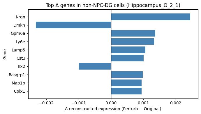
# ===== Visualization (bar plot) =====
# Visualize gene-wise changes in reconstructed expression
# after injection-based perturbation, excluding the target cell type.

import matplotlib.pyplot as plt

plt.figure(figsize=(7, 4))
plt.barh(df_delta["gene_symbol"], df_delta["delta_expr"], color="steelblue")
plt.axvline(0, color="black", lw=1)
plt.xlabel("Δ reconstructed expression (Perturb − Original)")
plt.ylabel("Gene")
plt.title(f"Top Δ genes in non-{target_celltype} cells ({target_slice})")
plt.gca().invert_yaxis()  # show top-ranked genes at the top
plt.tight_layout()
plt.show()

[INFO] Excluding target cell type: NPC-DG
[INFO] Remaining cells: 948 (original), 467 (perturbed)
                  gene_id gene_symbol  ori_mean_expr  perturb_mean_expr  \
13161  ENSMUSG00000053310        Nrgn       0.587867           0.590324   
4829   ENSMUSG00000060962        Dmkn       0.600472           0.598147   
9538   ENSMUSG00000031517       Gpm6a       0.438859           0.440233   
11551  ENSMUSG00000022587        Ly6e       0.479227           0.480565   
11148  ENSMUSG00000027270       Lamp5       0.445860           0.446925   
4232   ENSMUSG00000027447        Cst3       0.190023           0.191034   
10587  ENSMUSG00000001504        Irx2       0.194393           0.193402   
15191  ENSMUSG00000027347     Rasgrp1       0.361396           0.362378   
11682  ENSMUSG00000052727       Map1b       0.411003           0.411949   
4073   ENSMUSG00000033615       Cplx1       0.417111           0.418057   

       delta_expr  abs_delta  
13161    0.002457   0.002457  
4829    -0.002325   0.002325  
9538     0.001374   0.001374  
11551    0.001338   0.001338  
11148    0.001065   0.001065  
4232     0.001011   0.001011  
10587   -0.000990   0.000990  
15191    0.000982   0.000982  
11682    0.000946   0.000946  
4073     0.000945   0.000945

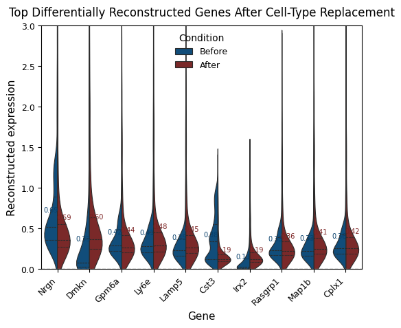
# ===== Select top genes by reconstruction change (|Δ|), top 20 =====
top_genes = (
    df_delta.sort_values("abs_delta", ascending=False)
    .head(20)["gene_symbol"]
    .tolist()
)

# Retrieve reconstructed expression matrices
X_ori = adata_ori.obsm["X_pred"]
X_perturb = adata_perturb_sub.obsm["X_pred"]

# Select indices of top genes
gene_idx = adata_ori.var["gene_symbol"].isin(top_genes)

expr_ori = X_ori[:, gene_idx]
expr_perturb = X_perturb[:, gene_idx]

# ===== Build plotting DataFrame =====
df_plot = pd.DataFrame(expr_ori, columns=adata_ori.var["gene_symbol"][gene_idx])
df_plot = df_plot.melt(var_name="gene_symbol", value_name="expr")
df_plot["condition"] = "Before"

df_plot2 = pd.DataFrame(expr_perturb, columns=adata_ori.var["gene_symbol"][gene_idx])
df_plot2 = df_plot2.melt(var_name="gene_symbol", value_name="expr")
df_plot2["condition"] = "After"

df_plot = pd.concat([df_plot, df_plot2], ignore_index=True)

# Ensure gene order follows Δ ranking
df_plot["gene_symbol"] = pd.Categorical(
    df_plot["gene_symbol"],
    categories=top_genes,
    ordered=True,
)

# ===== Violin plot =====
plt.figure(figsize=(5.5, 4.8))  # compact x-axis layout
sns.violinplot(
    data=df_plot,
    x="gene_symbol",
    y="expr",
    hue="condition",
    split=True,
    inner="quartile",
    palette={"Before": "#004f8bff", "After": "#871b1bff"},
    linewidth=0.8,
    scale="width",  # uniform violin width
)

# ===== Annotate mean expression values =====
means = (
    df_plot.groupby(["gene_symbol", "condition"])["expr"]
    .mean()
    .reset_index()
)

for i, gene in enumerate(top_genes):
    for cond, color in zip(
        ["Before", "After"],
        ["#073f6aff", "#791f1fff"],
    ):
        mean_val = means.query(
            "gene_symbol == @gene and condition == @cond"
        )["expr"].values[0]
        x_offset = -0.2 if cond == "Before" else 0.2
        plt.text(
            i + x_offset,
            mean_val,
            f"{mean_val:.2f}",
            color=color,
            ha="center",
            va="bottom",
            fontsize=7,
        )

# ===== Axis and style adjustments =====
plt.ylim(0, 3)  # fix y-axis range
plt.axhline(0, ls="--", c="gray", lw=1)
plt.xlabel("Gene", fontsize=11)
plt.ylabel("Reconstructed expression", fontsize=11)
plt.title(
    "Top Differentially Reconstructed Genes After Cell-Type Replacement",
    fontsize=12,
    pad=10,
)

plt.xticks(rotation=45, ha="right", fontsize=9)
plt.yticks(fontsize=9)
plt.legend(
    title="Condition",
    fontsize=9,
    title_fontsize=10,
    frameon=False,
)

plt.tight_layout(pad=0.8, rect=[0.02, 0, 1, 1])
plt.show()
# plt.savefig(
#     "violin_rec_exp_by_injected_theory2.pdf",
#     bbox_inches="tight",
#     dpi=300,
# )

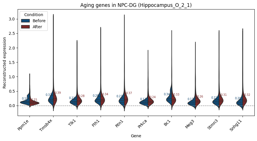
aging_genes = {
    "Bc1","Tlk1","Meg3","Ppm1e","Tmsb4x","Stmn3","Rtn1",
    "Prkca","Snhg11","Fth1"
}

# This block inspects reconstructed expression changes for a predefined set of
# genes of interest (aging-associated genes). By focusing on this curated gene set,
# the visualization highlights how biologically relevant aging markers respond
# to the perturbation in a targeted and interpretable manner.

# ==== Aging gene set ====
aging_genes = {
    "Bc1", "Tlk1", "Meg3", "Ppm1e", "Tmsb4x", "Stmn3", "Rtn1",
    "Prkca", "Snhg11", "Fth1",
}

# Retain only genes that are present in the current dataset
aging_genes_in_data = [
    g for g in aging_genes
    if g in adata_ori.var["gene_symbol"].values
]
print("Found aging genes:", aging_genes_in_data)

# ==== Retrieve reconstructed expression before and after perturbation ====
X_ori = adata_ori.obsm["X_pred"]
X_perturb = adata_perturb_sub.obsm["X_pred"]

# Select aging-associated genes
gene_idx = adata_ori.var["gene_symbol"].isin(aging_genes_in_data)

expr_ori = X_ori[:, gene_idx]
expr_perturb = X_perturb[:, gene_idx]

# ==== Build plotting DataFrame ====
df_plot = pd.DataFrame(
    expr_ori,
    columns=adata_ori.var["gene_symbol"][gene_idx],
)
df_plot = df_plot.melt(
    var_name="gene_symbol",
    value_name="expr",
)
df_plot["condition"] = "Before"

df_plot2 = pd.DataFrame(
    expr_perturb,
    columns=adata_ori.var["gene_symbol"][gene_idx],
)
df_plot2 = df_plot2.melt(
    var_name="gene_symbol",
    value_name="expr",
)
df_plot2["condition"] = "After"

df_plot = pd.concat([df_plot, df_plot2], ignore_index=True)

# Ensure gene order follows the predefined aging gene list
df_plot["gene_symbol"] = pd.Categorical(
    df_plot["gene_symbol"],
    categories=aging_genes_in_data,
    ordered=True,
)

# ==== Violin plot ====
plt.figure(figsize=(9, 5))
sns.violinplot(
    data=df_plot,
    x="gene_symbol",
    y="expr",
    hue="condition",
    split=True,
    inner="quartile",
    palette={"Before": "#004f8bff", "After": "#871b1bff"},
)

# Annotate mean expression values
means = (
    df_plot.groupby(["gene_symbol", "condition"])["expr"]
    .mean()
    .reset_index()
)
for i, gene in enumerate(aging_genes_in_data):
    for cond, color in zip(
        ["Before", "After"],
        ["#073f6aff", "#791f1fff"],
    ):
        mean_val = means.query(
            "gene_symbol == @gene and condition == @cond"
        )["expr"].values[0]
        x_offset = -0.2 if cond == "Before" else 0.2
        plt.text(
            i + x_offset,
            mean_val,
            f"{mean_val:.2f}",
            color=color,
            ha="center",
            va="bottom",
            fontsize=7,
        )

plt.axhline(0, ls="--", c="gray", lw=1)
plt.xlabel("Gene")
plt.ylabel("Reconstructed expression")
plt.title(f"Aging genes in {target_celltype} ({target_slice})")
plt.xticks(rotation=45, ha="right")
plt.legend(title="Condition")
plt.tight_layout()
plt.show()

Found aging genes: ['Ppm1e', 'Tmsb4x', 'Tlk1', 'Fth1', 'Rtn1', 'Prkca', 'Bc1', 'Meg3', 'Stmn3', 'Snhg11']